
Every click, scroll, and purchase leaves a trace. The more of these traces a Machine Learning (ML) model can study, the sharper its predictions and the stronger its commercial returns. The challenge is that no single organisation holds the full picture. The data is split across agencies, brands, and technology partners, each sitting on their own piece of the puzzle.
In our earlier work, we laid the groundwork for a federated way for organisations to collaboratively train a shared ML model for media performance, without having to centralize all their data puzzle pieces in one place. Each participant trains locally within their own infrastructure, and exchanges only model updates (weights) rather than raw data.
We then tested this idea with a set of experiments on simple ML models, comparing a centralised baseline (pooling everyone’s data in the same place and training a model on the full puzzle) with a federated counterpart that keeps the puzzle distributed across several data nodes. Alongside this, we examined how fragmentation to an increasing number of participating nodes affects overall performance.
Those initial experiments rested on two assumptions:
- All the data puzzle pieces look alike. Conceptually, this assumes that every data partner observes and records similar patterns and behaviors. This is a simplification of the real-world, where brands, agencies, and platforms address a diverse spectrum of audiences, products, and experiences.
- The federated ML model follows a traditional “tabular” architecture. Every row in its input is an observation (e.g. a marketing campaign), every column is a an aspect of that observation (e.g. the targeted audience, the advertised product). The last column is the outcome we are trying to model (e.g. the campaign’s performance). The model then looks for statistical associations among the columns from scratch, without having its own prior knowledge of the world. Again, this is a simplification of today’s AI/ML model landscape, where LLMs with vast prior world knowledge dominate.
In this next phase of our work, we relax both of these assumptions by exploring:
- Federated Learning in the presence of nodes with heterogeneous datasets
- Federated Fine-tuning of LLM-based predictive models
Contextualising the data: Marketing campaigns
Before turning to the experiments, it helps to revisit what the marketing dataset represents and where it comes from. We use synthetic datasets generated by a purpose-built pipeline designed to mirror the dynamics of real marketing campaigns. This approach gives us fine-grained control over each dataset’s composition, allowing us to construct targeted scenarios that stress-test the model under controlled conditions while retaining full visibility into the factors that drive campaign outcomes.
At the heart of this pipeline is a signed marketing knowledge graph, which encodes how marketing attributes interact. Each node is an attribute value—the brand being promoted, the audience it targets, the content’s creative tone and style, the platform it runs on, or the geography it reaches—and each edge captures whether two attributes are compatible (positive signal), incompatible (negative signal), or unrelated (missing signal).
This graph is the ground truth from which we sample subgraphs to build various synthetic datasets. Each dataset contains campaigns defined as combinations of these attributes: one brand, one audience, one creative (image or video), one platform, and one geographical location, drawn from the graph. Labels follow from the signals linking them: campaigns built from compatible pairings tend to over-perform (Positive), those from incompatible ones tend to under-perform (Negative), and mixed cases fall in between (Average). For full details on how the graph is built and sampled, see the synthetic data generator pod.
Generating heterogeneous data
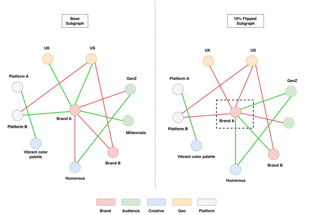
For our experiments, we utilised the ground-truth graph to extract four subgraphs for four respective datasets. To meet the requirement of using heterogeneous datasets, we deliberately add structural noise by randomly “flipping” the connected edges of a subset of subgraph nodes from positive to negative and vice versa. Figure 1 illustrates this on a sample subgraph: the left-hand panel (“Base Subgraph”) shows it in its original state. The right-hand panel (“10% Flipped Subgraph”) then shows a flip in action: we randomly select a fraction of nodes (here Brand A, boxed by the dashed rectangle) and reverse the signal on every edge connected to them, turning positive (green) edges negative (red) and vice versa. The result is a graph that tells a partly contradictory story, simulating the noisy, conflicting evidence of real marketing data.
The dataset names follow directly the fraction of nodes flipped, represented as percentage in each name. More specifically:
- Base (0%) leaves the graph untouched as a clean reference
- 10% Flip reverses a random 10% of nodes (the case in Figure 1)
- 20% Flip and 50% Flip apply the same step to larger fractions, adding steadily more noise
Since every dataset shares one origin and differs only in flip rate, this provides a controlled way to observe how the model copes as conflicting evidence accumulates—each dataset large enough to reach stable performance even without training to full equilibrium.
From tables to text: Federated LLM fine‑tuning with LoRA
The synthetic datasets start out as tables, where each row is a single campaign described by its features (brand, geography, audience, platform, and creative), and the last column records how that campaign performed—Positive, Negative, or Average. To prepare the data, we first replace these three labels with simple number codes (0, 1, or 2). We then treat the problem as a text classification task, where the model’s job is to read a campaign and produce a single answer at the end indicating its predicted performance.
Before training, every dataset goes through the same preparation steps, so all the inputs look consistent. Each campaign row is rewritten as a short, plain-language description that the LLM model can read, with each feature clearly labelled. For example, one campaign might look like this:
Platform: Platform A
Brand: Premium outdoor apparel brand
Audience: Young professionals interested in fitness and travel
Creative: Humorous
Geo: [1023, 2045, 9876] # Zip codes expression of the place
This description is then placed inside a fixed set of instructions that presents the task in exactly the same way for every experiment. During training, we include the correct performance label so the model can learn the patterns. During testing, we leave the label out, and the model has to work it out on its own—deciding whether the campaign is Positive, Negative, or Average.
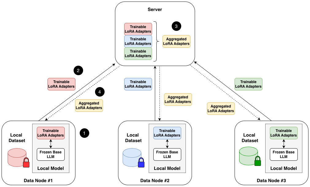
We recast the marketing problem as a task an LLM can solve, enabling us to fine-tune an LLM in a federated setup using FlowerTune with LoRA (Low-Rank Adaptation). We chose this approach because marketing data is typically sensitive and siloed across data nodes, and a federated setup keeps that data private: the model is trained locally at each node, so only the resulting updates—never the raw data—are ever shared. FlowerTune, the LLM fine-tuning tool in the Flower federated-learning framework, coordinates this process, while LoRA makes it practical: rather than exchanging billions of parameters each round, LoRA freezes the base model and trains only a small set of adapter weights, reducing the trainable parameters by over 99% and keeping communication cheap. As illustrated in Figure 2, a single communication round then proceeds in four steps: (1) Local training: each data node freezes the massive pre-trained base model and updates only the small set of LoRA adapters on its private, siloed dataset, so the raw data never leaves the node; (2) Upload updates: each node sends only these lightweight adapters—not the raw data or the full model—to the central server; (3) Aggregation: the server combines the adapters from all participating nodes into a single set of aggregated LoRA adapters, producing one shared, improved model; and (4) Broadcast: the server distributes these aggregated adapters back to every node to serve as the starting point for the next round. This cycle repeats over successive communication rounds until the model converges.
Experiments & lessons learned
For our experimental setup, we evaluate our text classification task using two LLMs of increasing size: Gemma-3-1b-it and Llama-3-8B-Instruct (1 billion and 8 billion parameters, respectively). Working with two models of different scale lets us assess not only the centralised-versus-federated gap, but also whether model capacity influences how gracefully each setup absorbs heterogeneous data.
For each model, we compare a centrally-trained LLM against its federated-trained counterpart across three progressively more heterogeneous settings:
- Setting 1 (2 Data nodes): The centralised model is trained on the combined samples of the Base and 10% Flip datasets. The federated equivalent uses two data nodes, one holding Base and the other 10% Flip.
- Setting 2 (3 Data nodes): The 20% Flip dataset is added, to the centralised training pool, and as an additional federated data node.
- Setting 3 (4 Data nodes): The 50% Flip dataset is added in the same manner, giving the most heterogeneous configuration.
All models are evaluated on a single, universal test set containing equal numbers of samples from every distribution (Base, 10%, 20%, and 50% Flip). This common benchmark provides a consistent view of how well each trained model generalises across the full spread of perspectives present in the federation. Each centralised scenario was trained for two passes over its own data; similarly each federated experiment used two communication cycles: in each cycle, every data node trained the model locally for one pass over its own data, then sent only the resulting model update to the server, which combined the updates before starting the next and final cycle, keeping total training exposure comparable between the two regimes. All other training parameters remain the same across the centralized version and its federated counterpart.
All models are evaluated on a single, universal test set containing equal numbers of samples from every distribution (Base, 10%, 20%, and 50% Flip). This common benchmark provides a consistent view of how well each trained model generalises across the full spread of perspectives present in the federation. Each centralised scenario was trained for two passes over its own data; similarly each federated experiment used two communication cycles: in each cycle, every data node trained the model locally for one pass over its own data, then sent only the resulting model update to the server, which combined the updates before starting the next and final cycle, keeping total training exposure comparable between the two regimes. All other training parameters remain the same across the centralized version and its federated counterpart.
Centralised vs. federated: The cost of heterogeneity
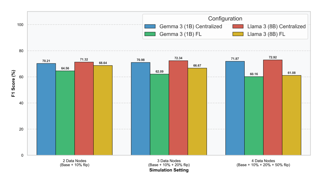
Gemma-3-1b-it and Llama-3-8B-Instruct models.Figure 3 reports the resulting F1 scores for Gemma-3-1b-it and Llama-3-8B-Instruct, respectively spanning all three settings. As anticipated, the centralised model outperforms its federated counterpart in every setting. This is an expected outcome, since centralised training enjoys unrestricted access to all data at once. One clearer pattern, however, emerges as the experiments scale.
The two regimes (centralized and federated) move in opposite directions**.** As more data is folded into the centralised pool, its overall score holds steady or even edges upward (for Gemma, from 70.21 → 70.98 → 71.87; for Llama, from 71.32 → 72.34 → 72.92). The federated model does the reverse: its score declines progressively as each new, more divergent data node joins (for Gemma, 64.56 → 62.09 → 60.16; for Llama, 68.64 → 66.67 → 61.08). In other words:
Additional data seems to be an asset when pooled centrally, but a growing liability when it arrives as conflicting federated contributions.
To understand why, it helps to look more closely at how the federated server combines what its data nodes send back. The aggregation method we use here is FedAvg (Federated Averaging), the standard baseline in federated learning: after each round, the server takes the model updates returned by every data node and averages them into a new shared model. This works well when data nodes hold similar data, because their updates broadly agree and reinforce one another. In our setup, however, each data node learns from a deliberately different distribution, so their updates pull in different—sometimes opposing—directions. Averaging then cancels out these distribution-specific signals, leaving a global model that is a bland compromise, serving no single distribution well. This is why federated performance erodes on a universal test set drawn from all distributions, and why that erosion deepens as we add data nodes that diverge ever further from the rest.
Lesson Learned: Standard federated learning is not a drop-in replacement for centralised training under heterogeneous data: as data nodes diverge, naïve FedAvg averaging cancels out their conflicting updates, so more participants can lower performance rather than raise it.
Our ongoing work in this space is now exploring alternative federated techniques that can overcome this limitation.
The effect of model scale under federation
Looking beyond the headline F1 comparison, we now turn to a more specific question: how does LLM’s size affect performance on this text-classification task under federation? The scores reported so far have been macro F1 scores, that is, the unweighted average of the F1 achieved on each of the three performance classes (Positive, Negative, and Average), treating every class as equally important regardless of how many samples it contains.
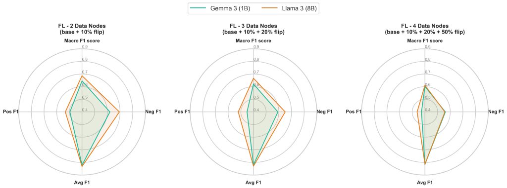
A single macro F1 figure is convenient for ranking configurations, but it hides where a model succeeds or struggles. Two models can reach the same macro score while being strong on different classes. To look underneath that average, Figure 2 decomposes performance for the three federated settings, plotting the macro (Total) F1 alongside the three per-class scores (Positive, Negative, and Average F1) for both models on a single radar chart. The three panels are ordered left to right by increasing heterogeneity, letting us see not just whether each model degrades, but which classes drive that decline.
Gemma-3-1b-it and Llama-3-8B-Instruct.Llama’s greater capacity appears to absorb mild and moderate heterogeneity more gracefully, reconciling divergent data node updates that a smaller model cannot: as Table 1 shows, at two data nodes its centralised–federated gap is less than half of Gemma’s (2.68 versus 5.65), and it remains markedly smaller at three nodes (5.67 versus 8.89). This advantage, however, does not persist indefinitely. Once the adversarial 50% Flip dataset enters the federation at four data nodes, both models degrade sharply and their gaps converge almost exactly (11.71 versus 11.84). The implication is clear:
Greater model capacity provides meaningful resilience to heterogeneity, but even a state-of-the-art model reaches a breaking point when a sufficiently divergent data node is introduced.
| Experimental setting | Gemma 3 (1B) Gap | Llama 3 (8B) Gap |
|---|---|---|
| 2 Data Nodes | 5.65 | 2.68 |
| 3 Data Nodes | 8.89 | 5.67 |
| 4 Data Nodes | 11.71 | 11.84 |
Table 1: Centralised–federated F1 gap for each LLM across the three experimental setups; a smaller gap indicates the federated model remains closer to its centralised performance.
Figure 4 makes this dynamic visible. In the two-node panel, the Llama-3 (8B) contour (orange) sits clearly outside the Gemma-3 (1B) contour (green) on every axis, evidence of the larger model’s stronger retained performance under mild heterogeneity. That margin narrows in the three-node panel as a more divergent data node joins, and nearly disappears in the four-node panel, where the 50% Flip data node pulls both contours toward the centre until they overlap, mirroring the convergence shown in the table. Because the radar chart separates the classes, it also reveals how the collapse occurs: both models maintain the same asymmetric profile throughout, extended toward Average F1 yet compressed at Positive F1. This indicates that, regardless of model size, FedAvg protects the Average class, while sacrificing the Positive class. Because the strong Average score inflates the macro average, the single headline F1 number hides this lopsided trade-off entirely.
Lesson Learned: Greater model capacity buffers heterogeneity but does not cure it: a larger LLM narrows the centralised–federated gap under mild and moderate divergence. Yet once a sufficiently adversarial data node joins, both models collapse similarly, because scale changes how much a model degrades, not how—leaving FedAvg’s aggregation as the true bottleneck.
The impact and looking ahead
Our experiments suggest a clear pattern: as more heterogeneous (non‑IID) data nodes join, federated performance declines.
What this implies:
- Heterogeneity is the driver: naïve federated aggregation averages conflicting updates, diluting distribution‑specific signals.
- A single “global” model may be the wrong target: when data nodes hold different “flavours” of data, a one-size-fits-all approach under-serves everyone.
Where we go next:
- Explore server-side strategies beyond naïve aggregation (FedAvg), e.g. personalisation methods that group data nodes by update similarity.
- Treat heterogeneity as a signal to exploit (discover who can beneficially collaborate), not just an obstacle.
Heterogeneity, it turns out, is not merely an obstacle to tolerate but a signal to exploit. Learning to harness it intelligently may ultimately determine how far federated learning can scale across the real, fragmented landscape of the marketing industry.
Disclaimer: This content was created with AI assistance. All research and conclusions are the work of the WPP Research team.
