Author: Emmanouil Kritharakis

Marketing organisations hold records of every campaign they have run, which can train models to predict how new plans will perform. But coverage is limited: each organisation has tried only a narrow range of campaigns, and none is willing to share records with competitors. Federated learning offers a way to train a shared model without moving anyone’s data, but it assumes all participants are solving the same problem. Organisations often aren’t: the same combination of audience, creative and platform can work well for one organisation and poorly for another, for reasons that are not apparent from either organisation’s data alone. Averaging their contributions can therefore produce a model that fits none of them; in our experiments, it reduced every participant’s accuracy. We show how to identify compatible partners in advance using only what participants already share during training, so no campaign records change hands. Averaging within clusters rather than across everyone improves the model of every organisation with a compatible partner.

Setting the problem

One of the most important questions in campaign planning is also the hardest: Will this work? Organisations already have the raw material to answer it. Every campaign they have run is documented by its brand, audience, format, platform and market, along with its performance. Those records can train a machine learning model to predict the outcome of a plan that has not yet run.

But predictive performance depends less on the model than on the records behind it. Most organisations work with a limited set of brands, a handful of audience segments, and a small number of platforms: a narrow slice of all possible campaigns. Asked about a combination beyond that experience, the model guesses. The experience of other organisations could close that gap.

The obvious solution is to pool data across organisations. The obvious obstacle is that nobody is willing to share raw data. Campaign performance data reveals what you spend, whom you target, and what actually works: three things you do not hand to a competitor. Data protection regulation also restricts organisations from sharing records containing personal data.

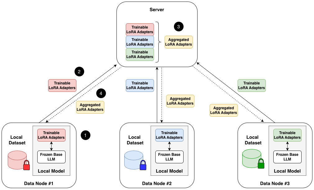
Federated Learning (FL) was designed for this challenge: the model moves to the data rather than the data moving to the model. A coordinating node sends the current model to each participant, which trains it on its own records and returns only the resulting parameter updates. The central node combines those updates into a model that, in theory, outperforms what any participant could build alone. We described this collaborative scenario for marketing records in an earlier post on fine-tuning a language model across organisations that keep their own data.

That earlier post left open the question that determines whether collaboration is worth joining: Are participants solving the same prediction problem? A model trained on campaign records maps campaign attributes to a verdict on performance. But that verdict is not an intrinsic property of a campaign; it reflects each organisation’s own benchmarks. As a result, two organisations can reach opposite conclusions about identical results. Their records then offer conflicting answers to the same question rather than complementary evidence about it.

Averaging updates in this situation pulls the shared model in opposing directions, producing a result that fits neither participant. In our experiments, every participant ended with a worse model than it would have had by training on its own records alone. This post describes two clustering methods for grouping compatible organisations before averaging. We show that the methods recover the intended grouping from the model updates participants already upload, and report their performance on a testbed built for that purpose.

Why naive averaging updates fails

The server combines orgnisations updates, weighting each by the number of records used for training. This is appropriate only if every organisation approximates the same target function: their updates are then independent estimates of the same quantity, and averaging reduces error.

That assumption fails in two distinct ways, each requiring a different remedy.

• Different outcomes for the same choices. A combination of campaign attributes that performs well for one organisation can perform poorly for another. The mapping from inputs to labels therefore differs between them, even when both describe campaigns identically and judge performance by the same standards.
• Different vocabularies. Each organisation describes campaigns in its own terms. Even when their tables have matching columns, the values may differ. Organisations may use different audience taxonomies, target different markets, or describe creative content in free text that a table cannot capture. As a result, the model’s inputs are not comparable across participants.

This post focuses on the first issue. Figure 1 illustrates a typical example.

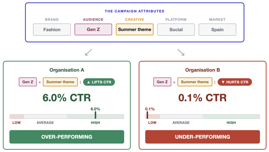
Two organisations run the same campaign, a summer-themed video advertisement for a fashion brand aimed at a Gen Z audience on one platform in one market. They describe the campaign with the same feature attributes, drawn from the same value space, and they judge the result by the same metric, click-through rate (CTR), and agree on which CTR values count as over-performing and which as under-performing. Organisation A measures a CTR of 6.0%, which both would call high. Organisation B measures 0.1%, which both would call low. Nothing about the description or the criteria differs, and the labels are opposite. This is known as “concept shift”: the mapping from inputs to labels differs between organisations [1], [2]. When the same combination of attributes leads to strong performance for one organisation and weak performance for another, averaging their updates does not reduce noise. Instead, it averages conflicting labelling functions, producing a result that fits neither.

The second issue, different vocabularies, can be addressed at the representation level. This is known as “covariate shift”: the distribution of the inputs differs between participants, while the mapping from inputs to labels stays the same [2], [4]. We replace the fixed table with free-text campaign descriptions and fine-tune a pre-trained large language model (LLM) with a prediction head. This offers two benefits. Differences in schema no longer disrupt training, because there is no schema to reconcile. The model’s existing knowledge helps it connect descriptions that a table would treat as unrelated: it can recognise that “Low-Income Millennials who enjoy hiking” and “Budget-conscious Gen Y trail walkers” describe much the same people, where a table sees two unrelated strings.

One important limitation: our experiments use a fixed input representation, with the same schema across all organisations. This article therefore addresses concept shift, not covariate shift. Testing covariate shift would require organisations whose attribute values genuinely differ, which is a direction for future work. Nevertheless, the free-text representation explains our choice of a language model as the baseline architecture.

Which participants to average, not how

Most published work on participant heterogeneity in federated learning changes how updates are combined: by keeping each participant close to the shared model [3], correcting for drift between participants [5], or adding a regularisation term to the local objective [6]. However, these methods cannot help when no single model fits every participant’s labels, as Figure 1 illustrates.

The real question is which participants should be averaged together. Participants whose criteria agree hold complementary evidence about one function and can usefully be averaged. Participants whose criteria conflict cannot, whatever the averaging rule. The server has to answer that without access to any participant’s records. All it receives is the parameter updates each participant uploads, so a usable method has to find compatibility in those.

What the uploaded model parameters contain

Full fine-tuning a pre-trained LLM and transmitting it every round is impractical, so we focus on a parameter-efficient fine-tuning (PEFT) method called Low-Rank Adaptation (LoRA), which freezes the pre-trained model and trains a pair of small adapter matrices, A and B, alongside it [7]. Participants exchange only those LoRA adapters, which are a small fraction of the model’s parameters.

The two matrices do different work. A holds general linguistic information, shared across participants because every participant describes campaigns in the same terms. B is task-specific: it holds the criteria by which a campaign record receives a performance label, and those criteria are what differ between participants. The same asymmetry is reported for low-rank adapters generally [8] and for federated fine-tuning in particular, where A carries knowledge transferable across clients and B carries what is specific to each one [9].

That asymmetry tells us which matrix to read, not which to share. Participants upload both, one of each for every layer of the model, and our methods use the B matrices to decide who is compatible with whom, then average the A and B matrices separately within each group that decision produces. The server already holds everything it needs as a normal part of training, so deciding which participants are compatible requires no campaign records and nothing beyond what federated training already sends.

How the server turns the LoRA adapters into groups

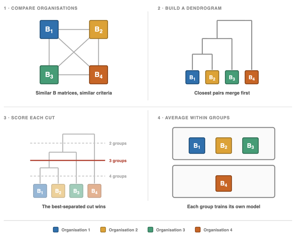
The server compares each organisation’s B matrices against every other’s. It measures how closely two organisations’ matrices align: closely aligned means the two are applying similar criteria, poorly aligned means they are not. Those comparisons are the only evidence the server has for forming the groups. Figure 2 shows the full sequence, from those comparisons to the final groups, and the rest of this section takes it step by step.

Building a hierarchy and choosing where to cut

From these comparisons, the server builds a hierarchy using agglomerative clustering. It starts with each participant in its own group and repeatedly merges the two closest groups until only one remains. The resulting tree does not prescribe a number of groups: cutting it high leaves everyone together, while cutting it lower divides them into two, three or more.

The key decision is where to cut, and the server makes it without being told how many groups to expect. It tests each candidate number of groups and scores the division in two ways. The Silhouette score [10] compares how close each participant is to its own group with how close it is to the nearest other group, rewarding clear membership. The Davies-Bouldin index [10] compares the spread within groups with the distance between them, penalising groups that are loose relative to the gaps separating them. A high Silhouette score and a low Davies-Bouldin index both indicate groups that are internally similar and clearly separated. The best-scoring division fixes the groups, and the decision is made once. In every round that follows, the server sends each group’s averaged adapter only to the organisations in that group, those organisations train locally and upload their updates, and the server averages them within the same groups again.

Two ways to apply the grouping

We developed two versions of this approach, Model-Wise Clustering and Layer-Wise Clustering, both adapting existing work on clustering clients in federated LoRA. They differ in one respect: whether the hierarchy is cut once for the whole model, or cut again at every layer, so that groups divide as the model deepens. Figure 3 shows how each version assigns organisations to groups.

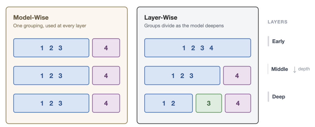
Model-Wise Clustering, influenced by [11], averages the comparisons across every layer into one distance per pair, builds a single hierarchy and cuts it once. Each organisation belongs to exactly one group, and that group decides which peers it is averaged with from the first layer to the last. The assumption is that an organisation’s criteria affect every layer to a similar degree.

Layer-Wise Clustering, influenced by [12], drops that assumption. The layers of the model do different work: the shallow ones handle general language that applies to any campaign description, while the deeper ones hold the mapping from a description to a performance label. It is that mapping which varies between organisations, so a single grouping applied throughout must either over-share in the deep layers or under-share in the shallow ones.

Layer-Wise therefore builds the same hierarchy, then walks the model from the first layer to the last, choosing at each depth how far down to cut. The evidence for each cut is the layer’s own distances, because two organisations can agree across the model as a whole and still diverge sharply at one depth. Because every cut comes from the same hierarchy, the groupings are nested rather than unrelated. Two rules govern the walk: the groups never merge back, so a divergence once detected holds deeper in, and a layer with no convincing split keeps the grouping of the one above it. The shallow layers stay unified and the groups divide as the model deepens, which is the pattern Figure 3 shows.

How we evaluated the two grouping methods

To judge a grouping, you have to know which grouping was right. A real federation never tells you: each participant’s criteria are private, so if accuracy changes, there is no way to attribute it to the grouping rather than to anything else. Therefore, we built a testbed where the answer is known in advance.

Generating campaign records from a rule graph

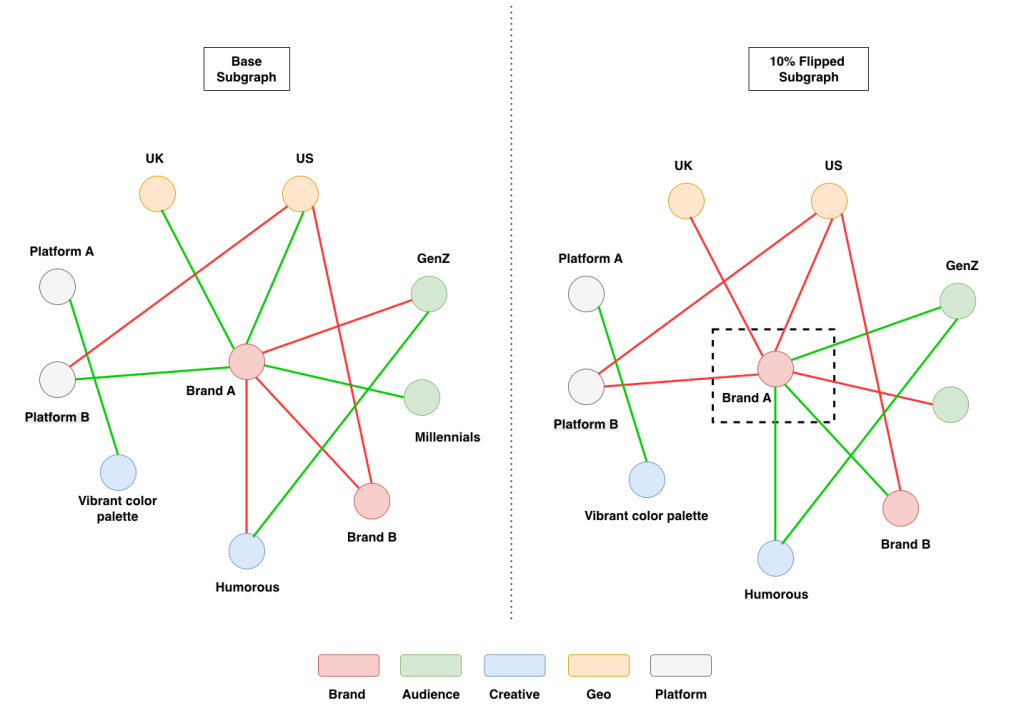
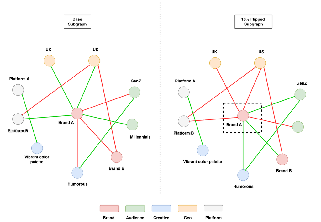
The testbed uses synthetic campaign records from a generator we built for this purpose, described in an earlier post on using synthetic data to stress-test marketing models. At its centre is a signed marketing knowledge graph, shown in the left panel of Figure 4. Each node is an attribute value, a brand, an audience, a creative treatment, a platform or a geography, and each edge records whether two of them work well together, shown in green, clash, shown in red, or have no bearing on each other.

A campaign record is one value of each kind, and its label follows from the edges between them: mostly green gives over-performing, mostly red gives under-performing, and mixed cases give average. We generated 27,000 records per organisation, split into a training set of 18,000 and a held-out test set of 9,000.

How the four organisations were made to disagree

We created four organisations and gave each a copy of the rule graph, flipping a controlled share of the nodes in three of the four. Flipping a node means changing the type of every edge incident to it, so that green becomes red and red becomes green. A campaign involving one of those choices then carries a different balance of green and red edges, and its label changes where that shift reverses the majority. The campaign records themselves are unchanged, so what differs between the four organisations is the labels alone. Figure 4 shows the base graph beside one of the three derived from it, with 10% of its nodes flipped.

Because we create the four graphs, we know the label each organisation’s criteria assign to every record it holds, and therefore how far any two organisations’ criteria diverge. Each organisation received a different share of flipped nodes. Table 1 gives the four organisations and how each one’s criteria relate to the original rules.

The four configurations span the range of disagreement we expect between advertising organisations. Two brands in adjacent categories agree about what a strong campaign looks like and differ at the margins. A brand with a different commercial model, a luxury house against a discount retailer, can reach the opposite conclusion from the same measured outcome.

Table 1 also fixes the grouping a method should produce. Organisations A, B and C belong in one group, because their criteria differ in degree rather than in kind and each holds records bearing on the others’ cases. Organisation D belongs on its own, because averaging its updates with the other three produces a model that fits none of the four. The sections that follow report which grouping each method produced.

Results

After federated training under each grouping strategy, we asked each organisation’s model two questions:

Does it work on your own campaigns? We trained each model on that organisation’s training set and tested it on its own held-out test set. This measures whether the model has learned that organisation’s own labelling criteria, the question an advertiser cares about day to day.

Does it generalise beyond your campaigns? We pooled the held-out test sets from all four
organisations into one large merged set (36,000 records) and tested each model against that. This measures whether a model has learned something about campaign performance in general, or has merely memorised one labelling criteria. It is the harder test, and it is the one that reveals whether collaboration delivered anything at all.

Both questions are scored with the same measure, the macro-averaged F1 score, reported as a percentage. It rewards a model for getting all three outcome campaign performance labels right (under-performing, average and over-performing), weighting the three equally, so failure on one cannot hide behind success on the others. Differences between approaches are quoted in percentage points.

Both methods recovered the intended grouping

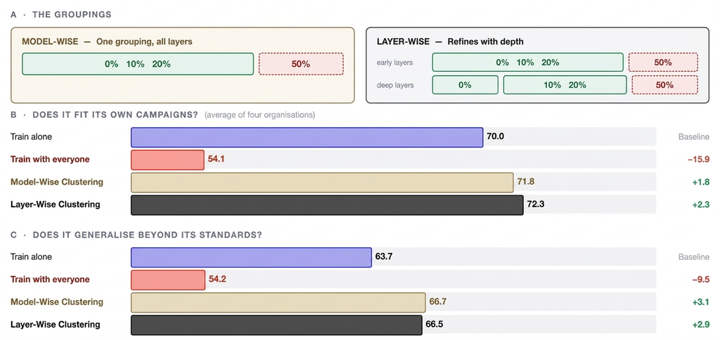
As panel A of Figure 5 shows, both placed the 50% organisation on its own and grouped the 0%, 10% and 20% organisations together, without access to any participant’s records. The server held nothing except the adapter matrices participants upload as part of training, and from the pair-wise similarities between those matrices it recovered the relationship between the four organisations’ labelling criteria, which it was not given.

The two methods then differ. Model-Wise applies that single grouping at every layer. Layer-Wise keeps it in the early layers and draws one further distinction in the deeper layers, separating the 0% organisation from the 10% and 20% pair, which matches the construction in Table 1: the three agree closely enough to share the layers that read a campaign and differ enough to separate in the layers that label it. That the distinction falls in the deeper layers is consistent with concept shift affecting the label rather than the reading.

On its own test set, each organisation scored at or above training alone

Panel B of Figure 5 reports each organisation’s model tested on its own held-out test set. Table 2 gives the individual scores behind those bars.

The first row of Table 2 shows that an organisation training alone scores between 59.0 and 78.4 depending on how self-consistent its own rulebook is, and those four figures average to 70.0. Two findings follow.

Clustering tracks each organisation’s own performance, and lifts it. Each clustering row follows the same shape as training alone, highest for the 0% organisation, lowest for the 50%, but sits above it at every point, gaining 1.8 points on average for Model-Wise and 2.3 for Layer-Wise. The margins are narrow, as expected of an organisation tested on its own campaigns with its full history available. What matters is the consistency: no organisation scored lower under either clustering method than it did training alone on its own test set.

Naive averaging loses to training alone for every organisation, by 15.9 points on average. This is the result that should give any prospective data collaboration pause. Every participant would have been better off never joining.

On the merged test set, clustering’s advantage over training alone grows

Panel C reports the same models on a single merged test set containing campaigns from all four organisations. This is a harder question, because three quarters of those campaigns are labelled by a standard the model was never trained on. Table 3 gives the individual scores behind panel C of Figure 5.

Every method scores lower here than on home ground, which is as it should be. Two further lessons follow.

The clustering advantage roughly doubles on the merged test. Clustering gains 3.1 points on average for Model-Wise and 2.9 for Layer-Wise, where naive averaging is 9.5 points behind. Compared with Table 2, the advantage is larger once models are asked to judge campaigns labelled by criteria other than their own. That is where collaboration is supposed to help, and where it does.

For the organisations that actually had partners, the gains are larger still. The averages in Table 3 include the 50% organisation, which by design had no partners. The three grouped organisations gained between 3.8 and 4.8 points over training alone: 66.3 rising to 70.1, 65.4 to 70.1, and 65.3 to 70.1. A model built on one dataset standard does not improve; one built on three related dataset standards does, because it has seen the same underlying dynamics judged in three slightly different ways and learned what they have in common.

What comes next

Compatibility determines which organisations can usefully train together, but not whether they should. In a real federation, access to a partner’s records comes at a price. Each organisation is both a seller, charging for access to its own records, and a buyer, using a fixed budget to acquire access to others’ data. Partner selection is therefore an economic as well as a statistical decision.

The methods described here address the statistical question: which participants are likely to benefit from training together? The next step is to give the server pricing information alongside the similarities it already computes, so it can form groups that deliver the greatest expected benefit to each participant within its budget. A partner who offers only a small improvement may not be worth the price, and the grouping that looks best by similarity may exceed every participant’s budget. We are now focused on extending these methods to partner selection under cost and budget constraints.

Conclusion

Federated learning creates value not by bringing more participants into the same model, but by ensuring that the right participants learn together. In our experiments, averaging updates from organisations with conflicting definitions of campaign success made every participant worse off than training alone, while clustering compatible organisations preserved or improved performance on their own campaigns and delivered larger gains beyond their home data. Crucially, the server identified those partnerships using only the LoRA matrices participants already upload, without seeing their campaign records, labels or business criteria. The practical implication is clear: privacy-preserving collaboration needs a compatibility step; the question is not whether more data helps, but whose data helps whom.

References

[1] Moreno-Torres et al. A Unifying View on Dataset Shift in Classification. In Pattern Recognition, 2012. https://doi.org/10.1016/j.patcog.2011.06.019

[2] Kairouz et al. Advances and Open Problems in Federated Learning. In Foundations and Trends in Machine Learning, 2021. https://arxiv.org/abs/1912.04977

[3] Li et al. Federated Optimization in Heterogeneous Networks. In MLSys 2020. https://arxiv.org/abs/1812.06127

[4] Zhu et al. Federated Learning on Non-IID Data: A Survey. In Neurocomputing, 2021. https://doi.org/10.1016/j.neucom.2021.07.098

[5] Karimireddy et al. SCAFFOLD: Stochastic Controlled Averaging for Federated Learning. In ICML 2020. https://arxiv.org/abs/1910.06378

[6] Acar et al. Federated Learning Based on Dynamic Regularization. In ICLR 2021. https://openreview.net/forum?id=B7v4QMR6Z9w

[7] Hu et al. LoRA: Low-Rank Adaptation of Large Language Models. In ICLR 2022. https://arxiv.org/abs/2106.09685

[8] Tian et al. HydraLoRA: An Asymmetric LoRA Architecture for Efficient Fine-Tuning. In NeurIPS 2024. https://arxiv.org/abs/2404.19245

[9] Guo et al. Selective Aggregation for Low-Rank Adaptation in Federated Learning. In ICLR 2025. https://arxiv.org/abs/2410.01463

[10] Davies and Bouldin. A Cluster Separation Measure. In IEEE Transactions on Pattern Analysis and Machine Intelligence, 1979. https://doi.org/10.1109/TPAMI.1979.4766909

[11] Wang et al. Adaptive LoRA Experts Allocation and Selection for Federated Fine-Tuning. In NeurIPS 2025. https://arxiv.org/abs/2509.15087

[12] Bian et al. FedTreeLoRA: Reconciling Statistical and Functional Heterogeneity in Federated LoRA Fine-Tuning. In ICML 2026. https://arxiv.org/abs/2603.13282

Disclaimer: This content was created with AI assistance. All research and conclusions are the work of the WPP Research team.

Why Federated Learning now?

In marketing, data is a competitive edge. The more audience signals, campaign performance data, and consumer behaviour a Machine Learning (ML) model can learn from, the sharper its predictions and the greater its business impact. Across the marketing ecosystem, spanning agencies, brands, and technology partners, organisations individually hold rich and valuable datasets. The potential to learn shared patterns across these assets, without ever exposing proprietary information, could unlock new capabilities: better audience targeting, smarter media spend, and faster creative optimisation at a global scale.

But here’s the challenge. Across the marketing industry, the most impactful data is inherently distributed. Each organisation, whether agency, brand, or technology partner, holds a unique piece of the data puzzle. Client contracts, privacy regulations like GDPR, and the sheer sensitivity of consumer-level data mean this data has to stay within each organisation’s walls. This is a structural reality of the industry, not a limitation of any single company. The question is whether there is a way to learn collectively from this distributed knowledge without compromising the privacy boundaries that exist for good reason.

The traditional solution, centralised ML, pools raw data from multiple sources into a single cloud to train a global model. But uploading terabytes of sensitive data to a central server creates severe network latency and exposes collaborators to data breaches and potential violations of privacy regulations.

Distributed ML methods attempted to address this by splitting training across local worker nodes. Whilst this reduces latency and avoids centralising raw data, these architectures were designed for internal computing clusters, not secure collaboration between independent companies. Without cross-organisation coordination, each organisation’s models are limited to what their own data can teach them, with no mechanism to benefit from shared learning.

Problem: The collaboration vs. privacy bottleneck

Organisations face a fundamental tension: gaining the benefits of shared learning typically requires centralising sensitive data, which privacy and contractual obligations rightly prevent. Yet without a way to learn collectively, each organisation’s models are limited to their own data alone. Neither traditional architecture offers a path to collaborative model improvement whilst keeping private data strictly where it belongs.

Federated Learning (FL) offers a way out of this dilemma by bringing the model to the data, rather than the other way around. To understand why this shift matters, let’s look at how FL actually works under the bonnet.

How Federated Learning works

Figure 1: Overview of the Federated Learning communication cycle between a central node and distributed client nodes.

Federated Learning (FL) enables multiple organisations to collaboratively train a shared model without ever centralising raw data. Instead of moving data to the model, FL brings the model to the data. Training proceeds through iterative rounds:

1. A central server sends the current global model to all participating nodes (Blue arrow).
2. Each node trains the model locally on its own private data (Green arrow).
3. Nodes send back only their model updates, never the underlying data (Pink arrow).
4. The server aggregates these updates into an improved global model and starts the next round.

Throughout this process, raw data never leaves its source. Only learned model representations are exchanged across the network.

The multimodal challenge

Whilst the above privacy-preserving framework is valuable in its own right, modern marketing data adds another layer of complexity. Organisations do not just work with spreadsheets and numbers. They work with images, video, text, audio, and structured data, often all at once. A single campaign might involve visual brand assets, ad copy, audience segments, and performance metrics across channels. Training models that can reason across these different data types, known as multimodal learning, is already one of the most demanding challenges in ML.

Now combine that with the constraints of federated learning. Each client may hold different combinations of modalities, in different formats and volumes. One partner might contribute rich visual data, another mostly text and tabular records. Coordinating a single global model that learns effectively from this fragmented, heterogeneous landscape, without ever seeing the raw data, pushes the problem to a new level of complexity.

This is precisely what makes the intersection of FL and multimodal learning so important, and so hard. If it can be made to work, it unlocks collaborative intelligence across organisations at a scale that neither approach could achieve alone.

Our objective: can Federated Learning deliver?

The promise of FL is compelling, but before investing in real-world deployment, we need to answer a fundamental question:

Does federated learning actually work well enough on multimodal marketing data to justify the tradeoff?

Centralised training will always have an inherent advantage, it sees all the data at once. The question is not whether FL can beat centralised performance, but whether it can get close enough to make the privacy and collaboration benefits worthwhile. And beyond raw performance, we need to understand how FL behaves under realistic stress conditions: more partners joining, noisy data, and complex cross-modal relationships.

To answer this, we designed a series of experiments around four key questions:

Experiment 1 — Centralised vs. federated performance

• How close can FL get to centralised performance? In a centralised setup, the model sees all the data at once, the ideal scenario for learning. FL, by design, fragments this data across nodes. The first question is whether this tradeoff costs us meaningful accuracy, or whether FL can match centralised results despite never accessing the full dataset.
• What happens as more clients join? In practice, a federated network might involve a handful of partners or dozens. As the number of participants grows, each node holds a smaller, potentially less representative slice of the overall data. We tested how model performance scales as we increase the number of nodes.

Experiment 2 — Resilience to noisy data

• How robust are centralised and federated models to noisy data? Real-world datasets are messy, labels can be wrongly defined, and data quality varies across partners. We deliberately introduced noise into the multimodal dataset to simulate these imperfections and measure how much degradation the model can tolerate before performance breaks down.

Experiment 3 — Cross-modal relationships

• How sensitive centralised and federated models to underlying cross-modal patterns? Multimodal models learn by connections between different types of data. For example, a luxury brand might target a high-income audience through a premium creative tone on a specific platform. Some of these connections appear frequently in the data, whilst others are rare. We tested whether emphasising the most frequent cross-modal patterns in our synthetic data improves performance compared to emphasising the least frequent ones, helping us understand how much the model benefits from common, naturally occurring relationships versus rare, atypical ones.

The data

For our experiments, we used a multimodal synthetic dataset generated by our own well-tested synthetic data generator, designed to mirror real-world marketing dynamics. The generator allows us to customise various elements of the data and design targeted datasets that stress-test our model architecture under controlled conditions, giving us full visibility into the factors that drive campaign performance.

Each campaign in the dataset is described using five key modalities:

• Audience – the consumer segment being targeted
• Brand – the positioning and perception of the brand
• Creative – the tone and message of the campaign
• Platform – where the campaign runs
• Geography – the markets being targeted

Each dataset’s sample is assigned a target label, Positive (Over performing), Negative (Under performing), or Average (Average performance), indicating whether that particular combination of modalities would lead to a successful, underperforming, or average campaign outcome.

Experimental results

All federated experiments are implemented using Flower, a widely adopted open-source framework for federated learning research and deployment. Flower allows us to simulate multi-client federated setups in a controlled environment, making it possible to rigorously test different configurations before moving to a fully distributed architecture.

To ensure a fair comparison between centralised and federated setups, we kept the playing field level. Both setups use the exact same model architecture, so any performance differences come from how the model is trained, not what is being trained. In the federated setup, data is split equally across nodes, so that each partner sees a representative sample. This way, when we increase the number of nodes, any change in performance can be attributed to the scaling itself, not to differences in what each node’s data looks like.

Experiment 1: How much accuracy do we trade for privacy?

Figure 2: Impact of increasing node fragmentation on Federated Learning performance. Performance clearly degrades as the number of nodes increases from 5 to 15, compared to the baseline centralised model version.

The centralised model sets the performance ceiling at 79.67%. This is expected, when a single model has direct access to all the data at once, it has the best possible conditions to learn. No information is lost to partitioning, and no coordination overhead is introduced. It’s the ideal scenario, and the benchmark everything else is measured against.

The federated results tell a clear story: as we add more nodes, performance gradually declines. With 5 nodes, the model reaches 76.23%, a modest drop from the centralised baseline. But as we scale to 10 and then 15 nodes, scores fall to 70.29% and 67.65% respectively. The same pattern holds across all metrics, with the sharpest drops in the model’s ability to correctly identify both positive and negative cases.

Why does this happen? As more nodes join, the total dataset gets divided into smaller slices. Each node sees less data, which means each node’s local training produces a less reliable picture of the overall patterns. When the server combines these local updates, the differences between them make it harder to converge on a strong global model, an effect we call the “aggregation penalty.”

Lesson learned: FL with 5 nodes comes remarkably close to centralised performance, showing that federated collaboration is viable with minimal accuracy loss. However, as the number of nodes grows, makes it progressively harder for the global model to match centralised results.

Experiment 2: How robust are centralised and federated models to noisy data? 

In practice, marketing data is never perfectly clean. Campaign outcomes don’t fall neatly into “this worked” or “this didn’t.” Was a campaign that slightly exceeded expectations truly a success, or just average? Was a modest underperformance a failure, or noise in the measurement? Different teams may label the same outcome differently, tracking systems introduce inconsistencies, and the line between a “positive” and “average” campaign is often blurry.

To simulate this reality, we deliberately introduced noise into our synthetic dataset by blurring the boundaries between performance classes. With no noise, the labels are clean — positive, negative, and neutral outcomes are clearly separated. As we increase the noise level from low, to medium, and then to high, the boundaries between these classes increasingly overlap, making it harder for the model to tell them apart. Think of it like gradually turning up the fog: the underlying patterns are still there, but they become harder to see. The federated learning simulation for this experiment was configured with 5 participating clients, consistent with the best-performing federated setup identified in Experiment 1.

Figure 3: Performance comparison of centralised (left) and federated learning (right) configurations across increasing noise levels. Both paradigms degrade gradually, with Positive F1 and Negative F1 most affected, whilst the performance gap between the two remains approximately constant across all conditions.

As expected, both models perform best on clean data and gradually decline as noise increases. At high noise:

• The centralised model’s score drops from 82.05% to 78.11%
• The FL model’s score drops from 80.74% to 76.09%

The good news: neither model collapses. Even at the highest noise level both models still perform reasonably well. The overall accuracy dips, and the models struggle most with distinguishing clearly positive or clearly negative campaigns, which makes sense, since those are exactly the boundaries we blurred. However, their ability to capture general patterns across the dataset remains stable throughout.

As in Experiment 1, the centralised model maintains a consistent edge over the federated setup at every noise level, but the gap between them stays roughly the same. This means that FL doesn’t become more fragile in noisy conditions; it handles data messiness about as well as its centralised counterpart.

Lesson learned: Real-world data is inherently noisy, and any viable model must be able to handle that. Both centralised and FL models show strong resilience — performance declines gradually rather than breaking down, even when the data is heavily corrupted. Importantly, FL’s relative performance holds steady across noise levels, suggesting it is no more vulnerable to messy data than centralised training.

Experiment 3: How sensitive are centralised & federated models to underlying cross-modal patterns?

Our synthetic data generator creates campaign data based on a graph of relationships between five key factors: Audience, Brand, Creative, Platform, and Geography. Each relationship captures whether a particular combination of these factors tends to drive strong or weak campaign performance. Some of these relationships are common and obvious — they show up frequently and reflect well-known marketing dynamics. Others are rare and subtle — unusual combinations that don’t appear often but may carry uniquely valuable signal about what makes a campaign succeed or fail.

Understanding how these different types of patterns affect learning is important for both training paradigms. If the nature of the underlying data patterns matters, we need to know whether centralised and federated models respond to them in the same way — or whether one setup handles certain patterns better than the other. To investigate this, we generated three versions of our dataset, keeping everything else the same:

• Common-first: The generator focuses on the most frequently occurring combinations and downplays the rarest ones. This gives us a dataset dominated by typical, familiar marketing patterns.
• Rare-first: The opposite — the generator prioritises the rarest combinations and downplays the most common. This fills the dataset with unusual, less obvious patterns.
• Middle-ground: The generator focuses on combinations that fall in the middle of the frequency spectrum, neither the most common nor the rarest.

As in Experiment 2, the federated learning simulation was run with 5 participating nodes, and performance was compared against the centralised baseline across all three dataset versions.

Figure 4: Impact of cross-modal relationships on model performance. Prioritising rare feature combinations (Rare-first) substantially improves accuracy compared with focusing on common patterns, showing that atypical relationships provide a stronger learning signal for both centralised and federated learning paradigms.

The results were striking. The Rare-first configuration dramatically outperformed the other two, achieving peak scores of 94.41% (Centralised) and 93.43% (FL), compared to scores in the 86–88% range for the Common-first and Middle-ground setups.

This tells us something counterintuitive: the model learns far more from unusual feature combinations than from common ones. The typical, frequently seen patterns are in some sense “easy”, they don’t give the model much new information. But rare combinations force the model to learn more nuanced and distinctive boundaries between what makes a campaign succeed or fail.

As in previous experiments, the centralised model maintains a small edge over FL, but the ranking between dataset strategies stays the same in both setups. Whether training centrally or federally, prioritising rare patterns is the winning strategy.

Lesson learned: Not all data is equally valuable. Prioritising on rare, atypical feature combinations produces significantly better models than focusing mostly on common patterns. This has direct implications for how we design synthetic datasets: rather than mimicking the most typical marketing dynamics, we should deliberately include uncommon combinations to give the model a richer and more discriminative learning signal.

The impact and looking ahead

This work is just the initial spark for our federated learning efforts. Verifying that the centralised ML model performance our company provides is slightly degraded under a reasonable number of users opens the discussion about delivering ML solutions that address shared challenges among clients who are reluctant to share data to tackle a common industry problem. The FL approach allows companies to securely train a shared global model on their own datasets without the risk of data leakage throughout the training process.

Although Federated Learning has been an established collaborative learning method since 2017, it remains a highly active research domain in academia and a strategic priority for industrial implementation.

Our next objective is to stress-test and further expand our federated learning (FL) infrastructure by enabling learning across nodes that hold highly heterogeneous data, with substantially different shapes, feature spaces, and underlying distributions. This introduces a number of technical challenges, including how to align representations, aggregate knowledge effectively, and maintain stable performance when local data varies significantly from node to node. Overcoming these challenges will unlock deeper insights into the robustness and scalability of our FL framework, and will allow our models to learn more effectively in realistic, decentralised settings where data heterogeneity is the norm rather than the exception.

Ready to explore the specifics? Read our full technical deep dive into Multimodal Federated Learning for a closer look at our methodology.

Disclaimer: This content was created with AI assistance. All research and conclusions are the work of the WPP AI Lab team.