Author: Serafeim Papadias

Large language model routing aims to reduce inference cost and latency by matching each request to an appropriate model tier without materially degrading answer quality. This study compares three request-classification strategies: Gemini 2.5 Flash Lite, TypeSafe’s Jev, and LiteLLM’s default heuristic using simple, medium, and reasoning models. We evaluate each strategy on samples from four public datasets, measuring answer accuracy, classification and response latency, classification and response cost, and model-selection patterns. Our goal was to investigate whether routers can choose the right level of “brainpower” for each question instead of always relying on the most powerful and expensive model. Jev offered the strongest overall balance, making routing decisions faster and more cost efficient than Gemini while delivering broadly comparable accuracy. The results show that smarter routing can make AI applications faster and more affordable, although the best approach will depend on an organisation’s accuracy needs, budget, and data-privacy requirements.

Motivation – Allocating cognition at the request-level

In our previous article, Cost-Aware LLM Request Routing: From Tokenomics to Dynamic Cognitive Allocation [1], we examined why applications should allocate model capacity according to the requirements of each request. Model providers now offer LLMs with different levels of capability, latency, and cost. Sending every request to the most capable model can consume more time and money than the task requires. Sending every request to the cheapest model creates the opposite risk: difficult tasks may receive answers from a model that lacks the required reasoning capability.

An LLM router selects a model for each incoming request. In a fixed configuration, a developer chooses the model in advance, and every request follows the same route. Dynamic routing removes this assumption. The application has no a priori knowledge of which model a request requires, so the router classifies the request and assigns it to a capability tier, such as simple, medium, or reasoning. The router must balance three requirements:

• Accuracy measures whether the selected model answers the request correctly.
• Classification latency measures how much time the classification step adds before the selected model begins processing the request. Response latency measures the time required for an autoregressive model (LLM) to provide a full answer where reasoning models take longer.
• Cost includes both the classification step and the model that produces the answer.

Routing therefore introduces an additional step before the answer is generated. This step adds classification cost and latency, but it can reduce response cost and response latency by directing suitable requests to less expensive and faster models. A useful router must produce enough savings at the response stage to justify its classification overhead, without causing an unacceptable loss in answer accuracy.

In this article, we test three classification components for an LLM router: a lightweight LLM, Jev, and a keyword-based heuristic classifier. We compare their answer accuracy, classification latency, classification cost, response cost, and end-to-end response latency with fixed model selection.

Jev: Structured Decisions Without Text Generation

Jev [2] is TypeSafe’s first System One model. The name draws on the distinction between fast, intuitive System 1 thinking and slower, deliberate System 2 reasoning, popularised by Daniel Kahneman in Thinking, Fast and Slow [3]. In this context, System One refers to focused judgments that do not require a written explanation. Jev applies this approach to natural-language input and returns structured values that software can use directly.

This design differs from that of a conventional large language model. An LLM generates text one token at a time, even when an application only needs a category or score. The application must then parse and validate the generated text before it can act on the result. Jev does not generate a written response. It evaluates a defined question against the supplied state, which contains the request and any context needed to classify it, and returns an answer in a format specified by the application.

Jev exposes classification through question types called primitives. For LLM routing, the relevant primitive is Choice, which selects one option from a fixed set. In our router, the options are SIMPLE, MEDIUM, and REASONING. Each option represents a model tier with a different balance of capability, latency, and cost. Jev evaluates the incoming request against these options, and the application sends the request to the model assigned to the selected tier.

A Choice response contains three parts:

• choice identifies the selected model tier.
• probabilities reports the probability assigned to every available tier.
• confidence describes how strongly the probability distribution favours one option.

The distinction between probabilities and confidence matters when a request lies near the boundary between two tiers. A router can use a high-confidence classification directly and route a low-confidence request to a more capable model. Confidence does not guarantee that an individual decision is correct. TypeSafe describes Jev’s probabilities as calibrated across groups of predictions, meaning that higher probabilities should correspond to higher observed accuracy when results are evaluated over many requests.⁠

Jev’s suitability can be considered against the routing requirements introduced in the motivation:

• For accuracy, Jev’s probabilities and confidence expose uncertainty about the selected tier, while Choice ensures that the output is one of the permitted routing options. Whether those selections preserve answer accuracy must be determined from the responses produced by the selected models.
• For latency, Jev adds the time required to classify the request before the selected model can answer it. The relevant measurements are therefore the classification latency and the end-to-end response latency.
• For cost, Jev incurs a classification cost and influences the response cost through the model tier it selects. A lower classification cost does not by itself imply a lower combined cost; the classification and response costs must be considered together.

These properties explain why Jev is a plausible classification solution, but they do not establish whether it selects the appropriate tier or improves the balance between accuracy, latency, and cost. Our experimental evaluation using LiteLLM as the proxy service [4] tests this proposition. It begins with fixed-model baselines and then compares three routing strategies: an LLM classifier, Jev, and a keyword-based heuristic classifier.

Experimental evaluation over multiple routing strategies

Datasets

We evaluate the routing strategies on four evaluation sets with different reasoning requirements. The sets are derived from PIQA, WorldSense, and RouterBench. PIQA and WorldSense are available through Inspect Evals [5, 6, 8], while RouterBench combines questions from several established benchmarks [7].

The full evaluation sets contain between 1,838 and 40,176 questions. Each experimental condition uses a sample of 100 questions from each set. Table 1 summarises the available sample size, answer format, included content, and reasoning level assigned in our experimental design.

Table 1. Evaluation sets used in the routing experiments. Each experiment uses 100 sampled questions from each set.

Representative questions

The following examples illustrate the answer formats used in PIQA and WorldSense.

PIQA example

Input: Make outdoor pillow.
Choices: A: Blow into tin can and tie with rubber band. B: Blow into trash bag and tie with rubber band.
Target: B

WorldSense example

Input: There are three people of different heights in a room: Patricia is taller than Grace, and Patricia is taller than Robert. Choose one of the following alternatives: 1. Robert is taller than Grace. 2. Robert is shorter than Grace. 3. It is impossible to decide.
Choices: 1, 2, 3
Target: 3

The harder WorldSense subset contains two categories:

• completion problems asks which statement follows from a description and includes cases where the answer cannot be determined.
• normal contains questions that the evaluation describes as requiring a world model to solve.

RouterBench contains multiple-choice questions drawn from MMLU, HellaSwag, WinoGrande, and ARC-Challenge. The questions have two, three, or four possible answers.

Prompt format

We convert every question to the same prompt format so that responses can be parsed and evaluated consistently:

prompt = (
f"Input: {input_text}\n"
f"Choices: {choices}\n"
"Which choice is correct? "
"DO NOT try to explain your answer."
)

We instruct each model to return only the selected option so that answers can be parsed and evaluated consistently. This instruction limits the visible response, but provider-reported reasoning tokens, where applicable, remain part of the model usage and cost.

Before comparing the routing strategies, we establish fixed-model baselines to measure how the simple and reasoning models perform on these evaluation sets.

Baseline: pinned models

We first establish two fixed-model baselines. In each baseline, we pin one model in the LiteLLM proxy and use that model for every request. There is no classification step and no dynamic selection between models.

The first baseline uses gemini-2.5-flash-lite, which represents the simple tier. The second uses gemini-2.5-pro, which represents the reasoning tier. Both models come from the same provider and model family, limiting variation unrelated to the choice of model.

For each evaluation set, we randomly sample 100 questions and measure answer accuracy and the total wall-clock time required to process them. Requests are submitted with a concurrency of five.

A configuration consists of one model evaluated on one evaluation set. We evaluate each configuration over three independent runs. Across these runs, answer accuracy varies by approximately two percentage points, while wall-clock time varies by approximately 5%. Provider load is not controlled and may contribute to the observed timing variation.

Table 2 shows that gemini-2.5-pro achieves higher observed accuracy than gemini-2.5-flash-lite on all four evaluation sets. The observed difference is 9 percentage points on PIQA, 10 on RouterBench, 45 on WorldSense, and 35 on WorldSense completion and normal. These differences should be read alongside the run-to-run variation reported above.

The higher observed accuracy is accompanied by a substantial increase in processing time. gemini-2.5-flash-lite processes each evaluation set in 13.2 to 14.8 seconds, whereas gemini-2.5-pro, requires 170 to 193 seconds.

These fixed-model results provide reference points for the routing experiments. Sending more requests to gemini-2.5-pro may preserve or improve answer accuracy, but it also increases response latency and cost. Sending more requests to gemini-2.5-flash-lite reduces response latency and cost, but may reduce accuracy. The routing experiments test whether a classifier can manage this trade-off by selecting among the available model tiers for each request.

Smart routing, option 1: Gemini classifier

The first routing strategy uses a lightweight language model as the classifier. For each request, the classifier selects one of three available models. This is part of the LiteLLM configuration file:

tiers:

SIMPLE: gemini-2.5-flash-lite

MEDIUM: gemini-2.5-flash

REASONING: gemini-2.5-pro

classifier_llm_config:
model: gemini-2.5-flash-lite

The classifier uses gemini-2.5-flash-lite to evaluate the input and select a model. LiteLLM then sends the original request to the selected model.

The model selections are outputs of the classifier, not ground-truth labels. The experiments therefore do not measure whether the classifier selects an objectively correct model for each question. Instead, we evaluate the resulting system using final-answer accuracy, latency, cost, and the distribution of requests across the three models.

Figure 1 shows how the Gemini classifier distributes the 100 questions from each evaluation set. The panels follow the reasoning order established in Table 1: PIQA, RouterBench, WorldSense, and WorldSense completion and normal.

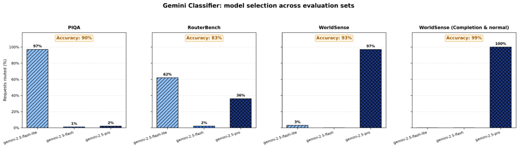
For PIQA, the classifier routes 97 of the 100 questions to gemini-2.5-flash-lite, 1 to gemini-2.5-flash, and 2 to gemini-2.5-pro. The resulting system answers 90 questions correctly. For RouterBench it produces a more varied distribution. The classifier routes 62 questions to gemini-2.5-flash-lite, 2 to gemini-2.5-flash, and 36 to gemini-2.5-pro. The resulting system answers 83 questions correctly. The distribution changes for the two hard WorldSense sets. The classifier routes 97 WorldSense questions to gemini-2.5-pro and all 100 questions from WorldSense completion and normal to that model. The resulting system answers 93 and 99 questions correctly, respectively.

Table 3 reports answer accuracy, model selection, classification cost and latency, response cost and latency, and output-token use. Classification measurements cover the routing decision, while response measurements cover the routed request and the selected model’s response. Cost, latency, and token measurements are reported per request. Total evaluation time is the wall-clock time required to process all 100 questions.

Table 3 shows that mean classification latency remains between 643 and 720 ms across the four evaluation sets. Mean classification cost similarly remains between $4.22e-05 and $5.10e-05 per request. The classification stage therefore introduces a relatively consistent measured overhead across these experiments.

Response latency and cost vary more substantially. PIQA has a mean response latency of 1,307 ms and a mean response cost of $1.20e-04 per request. These values increase to 4,959 ms and $0.0045 on RouterBench, 8,926 ms and $0.010 on WorldSense, and 10,135 ms and $0.012 on WorldSense completion and normal.

This variation accompanies the change in model selection shown in Figure 1. The Gemini classifier predominantly selects gemini-2.5-flash-lite for PIQA but predominantly selects gemini-2.5-pro for the two WorldSense sets. RouterBench falls between these cases, with requests divided mainly between the simple and reasoning models.

The output-token measurements follow a similar pattern. PIQA has a mean of 27 output tokens per request, compared with 462 for RouterBench, 942 for WorldSense, and 1,216 for WorldSense completion and normal. These are provider-reported usage measurements and should not be interpreted as visible answer length. The prompt instructs each model to return only the selected option, but provider-reported reasoning tokens, where applicable, remain part of model usage and cost.

The Gemini classifier provides a model-based reference for the remaining experiments. We next retain the same three downstream models and replace the Gemini classification step with Jev. This allows us to compare the two classifiers without changing the models available to the router.

Smart routing, option 2: Jev classifier

We next replace the Gemini classifier with Jev while retaining the same three downstream models. This allows us to compare the two classifiers without changing the models available to the router.

The experiments use Jev version 1.13.0, integrated through LiteLLM version 1.103.0rc01. The relevant LiteLLM configuration is:

tiers:

SIMPLE: gemini-2.5-flash-lite

MEDIUM: gemini-2.5-flash

REASONING: gemini-2.5-pro

classifier_type:
model: jev

jev_classifier_config:

model: jev-latest

Figure 2 shows how Jev distributes the 100 questions from each evaluation set. As in Figure 1, the panels are ordered by their assigned reasoning difficulty: PIQA, RouterBench, WorldSense, and WorldSense completion and normal.

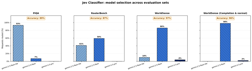
For PIQA, Jev routes 93 of the 100 questions to gemini-2.5-flash-lite and 7 to gemini-2.5-flash. The resulting system answers 89 questions correctly. For RouterBench, Jev divides the questions between the simple and medium models. It routes 41 questions to gemini-2.5-flash-lite and 59 to gemini-2.5-flash, producing 87 correct answers. For WorldSense, Jev routes 10 questions to gemini-2.5-flash-lite, 86 to gemini-2.5-flash, and 4 to gemini-2.5-pro. For WorldSense completion and normal, it routes 98 questions to gemini-2.5-flash and 2 to gemini-2.5-pro. The resulting system answers 97 and 96 questions correctly, respectively.

Table 4 reports the complete Jev results. As in Table 3, total evaluation time covers the complete run of 100 questions. Cost, latency, token, and confidence measurements are reported per request.

Comparison with the Gemini classifier

Figures 1 and 2 show different model-selection patterns. The Gemini classifier sends 97 WorldSense questions and all 100 WorldSense completion and normal questions to gemini-2.5-pro. Jev instead sends most questions from both sets to gemini-2.5-flash, selecting gemini-2.5-pro for only 4 and 2 questions, respectively.

This difference in model selection is accompanied by lower response cost. Compared with the Gemini classifier, Jev reduces mean response cost:

• From $1.20e-04 to $7.42e-05 per request on PIQA.
• From $0.0045 to $0.0013 on RouterBench.
• From $0.010 to $0.002 on WorldSense.
• From $0.012 to $0.003 on WorldSense completion and normal.

The reductions on the two WorldSense sets are fivefold and fourfold, respectively. The results do not support describing either reduction as an order of magnitude.

Jev also has lower mean response latency on all four evaluation sets. Compared with the Gemini classifier, mean response latency decreases from 1,307 to 1,020 ms on PIQA, from 4,959 to 3,245 ms on RouterBench, from 8,926 to 3,617 ms on WorldSense, and from 10,135 to 5,624 ms on WorldSense completion and normal.

These reductions are not accompanied by a consistent change in accuracy across all four sets.

Classification cost and latency are also lower with Jev. Its mean classification cost ranges from $2.15e-05 to $2.45e-05 per request, approximately half the corresponding Gemini classification cost. Its mean classification latency ranges from 235 to 274 ms, compared with 643 to 720 ms for the Gemini classifier. This corresponds to a reduction of approximately 60% to 65% across the four evaluation sets.

Classification confidence

Jev also returns a confidence value for each model selection. Mean confidence is 0.69 on PIQA, 0.59 on RouterBench, 0.54 on WorldSense, and 0.55 on WorldSense completion and normal. These confidence values expose information that is not available from a model-selection label alone. A production router could use confidence as an additional control signal, such as sending requests below a chosen threshold to a more capable model. This policy was not evaluated in the present experiments. Any threshold would need to be tested on representative application traffic because escalation could increase accuracy, latency, and cost.

Deployment consideration

Deployment architecture introduces an important privacy consideration. In these experiments, Gemini is hosted in the organisation’s Google Cloud environment, whereas Jev classification requires sending request content to TypeSafe’s external endpoint. This may be unsuitable for deployments involving confidential, regulated, or proprietary data unless the corresponding data-processing, retention, and residency requirements have been assessed. Jev’s lower classification cost and latency should therefore be evaluated alongside its security and governance implications.

Smart routing, option 3: Heuristic classifier

The default routing option for LiteLLM is the heuristic classifier, where no LLM is used for routing decisions. Instead, the heuristic classifier scores each request across seven dimensions and maps the score to a tier. These scores span token count, code presence, keywords associated with reasoning etc all of which are configurable by the user.

Unlike the Gemini and Jev classifiers, avoiding the invocation of a separate language model incurs no classification cost and adds marginal latency. Its effectiveness, however, depends on whether the configured rules provide a useful approximation of the capability required by each request.

For our test cases we opted for the default values and part of the LiteLLM configuration file related to tier boundaries is:

tier_boundaries:

simple_medium: 0.15

medium_complex: 0.35

complex_reasoning: 0.60

Because the heuristic does not invoke a separately billed classification model, it has no classification cost. It still introduces a small amount of classification latency while it evaluates the request and selects a model. Figure 3 shows how the heuristic classifier distributes the 100 questions from each evaluation set. The panels use the same difficulty order as Figures 1 and 2.

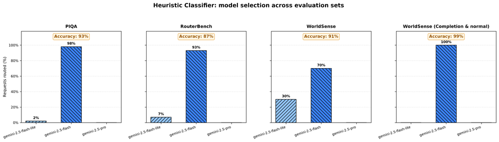
For PIQA, the heuristic routes 2 of the 100 questions to gemini-2.5-flash-lite and 98 to gemini-2.5-flash. The resulting system answers 93 questions correctly. For RouterBench, it routes 7 questions to gemini-2.5-flash-lite and 93 to gemini-2.5-flash. The resulting system answers 87 questions correctly. For WorldSense, the heuristic routes 30 questions to gemini-2.5-flash-lite and 70 to gemini-2.5-flash, producing 91 correct answers. For WorldSense completion and normal, it routes all 100 questions to gemini-2.5-flash, producing 99 correct answers. The heuristic does not select gemini-2.5-pro for any question in the four samples.

Table 5 reports the complete results. Total evaluation time covers the complete run of 100 questions. All other cost, latency, and token measurements are reported per request.

Classification overhead

The heuristic has the lowest classification overhead of the three routing strategies. Its mean classification latency ranges from 11 to 33 ms, compared with 235 to 274 ms for Jev and 643 to 720 ms for the Gemini classifier. It also has no separately billed classification cost.

Low classification overhead does not necessarily produce the lowest response latency or response cost. These measurements also depend on which downstream model the classifier selects. As Figure 3 shows, the heuristic sends most questions in every evaluation set to gemini-2.5-flash.

Comparison with Jev

The PIQA results illustrate the distinction between classification overhead and the performance of the complete routed request. The heuristic has a mean classification latency of 11 ms, compared with 235 ms for Jev. However, the heuristic routes 98 questions to gemini-2.5-flash, while Jev routes 93 questions to gemini-2.5-flash-lite.

In this sample, the heuristic produces 93 correct answers, compared with 89 for Jev. This increase is accompanied by a higher mean response cost and latency. Mean response cost increases from $7.42e-05 with Jev to $8.60e-04 with the heuristic, an increase of more than elevenfold. Mean response latency increases from 1,020 to 2,227 ms.

On RouterBench, both classifiers produce 87 correct answers. Jev routes 41 questions to gemini-2.5-flash-lite and 59 to gemini-2.5-flash, while the heuristic routes only 7 to gemini-2.5-flash-lite and 93 to gemini-2.5-flash. Jev has a lower mean response cost of $0.0013 per request, compared with $0.0016 for the heuristic. It also has a lower mean response latency of 3,245 ms, compared with 3,787 ms.

The pattern differs on WorldSense. The heuristic has a lower mean response cost and latency than Jev, but it produces 91 correct answers compared with 97 for Jev. On WorldSense completion and normal, the two classifiers have the same mean response cost. The heuristic produces 99 correct answers, compared with 96 for Jev, and has a slightly lower mean response latency.

These results do not establish that either classifier is preferable across all evaluation sets. They show that reducing classification overhead alone does not determine the cost, latency, or accuracy of the complete routed request.

Configuration considerations

The heuristic provides a low-overhead baseline that is deterministic for a fixed configuration. It also avoids sending a request to a separate classification service. Its results depend on the selected tier boundaries, feature weights, and routing keywords. The default configuration predominantly selects gemini-2.5-flash in these experiments and does not select gemini-2.5-pro. A different configuration could change the model-selection distribution and the resulting accuracy, latency, and cost.

Unlike Jev, the heuristic does not provide calibrated probabilities or a confidence value that could identify uncertain model selections. Its tier boundaries and scoring rules would therefore need to be evaluated and adjusted using representative application traffic.

The conclusion compares all three routing strategies across answer accuracy, classification latency, response latency, classification cost, and response cost.

Conclusions

Figures 1–3 show that the three classifiers produce substantially different model-selection patterns. The Gemini classifier frequently selects gemini-2.5-pro for the hard WorldSense sets. Jev predominantly selects gemini-2.5-flash for those sets and rarely selects gemini-2.5-pro. The heuristic also favours gemini-2.5-flash, but its model-selection distribution changes less across the four difficulty levels.

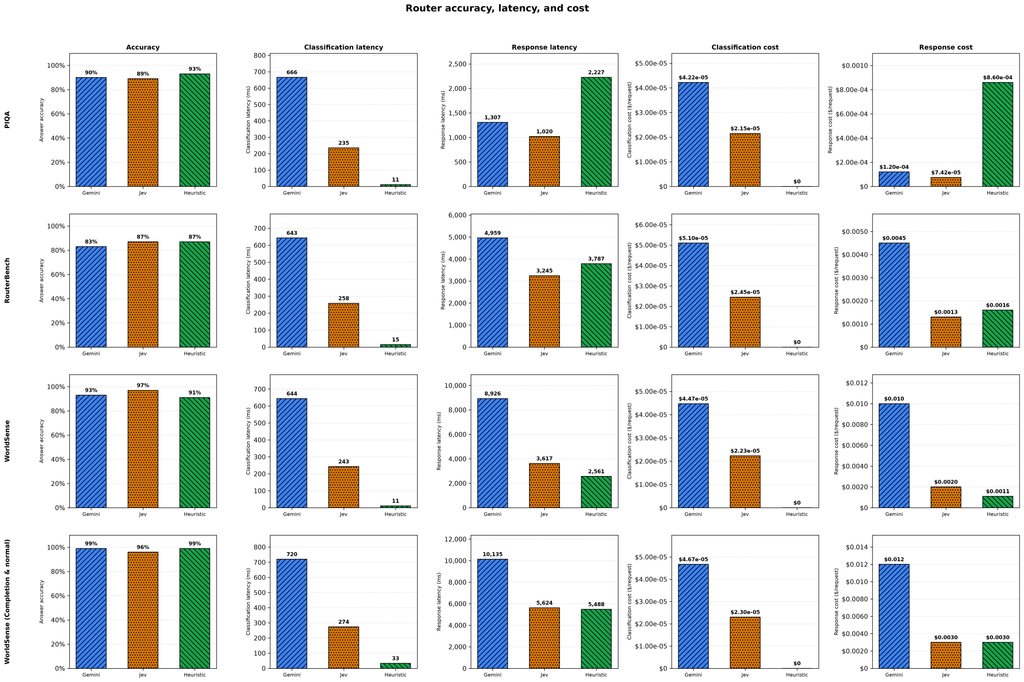
Figure 4 brings the five evaluation metrics together. Each row represents one evaluation set, ordered by its assigned reasoning difficulty. The columns compare answer accuracy, classification latency, response latency, classification cost, and response cost. Each panel contains one bar for the Gemini, Jev, and heuristic classifiers.

Gemini Vs Jev Routing

Figure 4 shows that Jev has lower classification and response measurements than the Gemini classifier across all four evaluation sets. Mean classification latency with Jev ranges from 235 to 274 ms, compared with 643 to 720 ms for the Gemini classifier. This represents a reduction of approximately 60% to 65%. Jev’s mean classification cost is also approximately half that of the Gemini classifier. The difference continues at the response stage. Compared with the Gemini classifier, Jev reduces mean response cost.

Jev also reduces mean response latency from 1,307 to 1,020 ms on PIQA, from 4,959 to 3,245 ms on RouterBench, from 8,926 to 3,617 ms on WorldSense, and from 10,135 to 5,624 ms on WorldSense completion and normal.

These reductions are accompanied by different accuracy results across the evaluation sets. Compared with the Gemini classifier, Jev produces one fewer correct answer on PIQA and three fewer on WorldSense completion and normal. It produces four more correct answers on both RouterBench and WorldSense.

The Gemini classifier’s higher cost and latency on the WorldSense sets accompany its frequent selection of gemini-2.5-pro. Jev instead routes most questions from these sets to gemini-2.5-flash. The results show that the more frequent use of the reasoning model does not produce higher aggregate accuracy on every evaluation set.

Jev Vs Heuristic Routing

The heuristic has the lowest classification latency and no separately billed classification cost. However, Figure 4 shows that reducing classification overhead does not necessarily minimise the cost or latency of the complete routed request. On PIQA, the heuristic produces four more correct answers than Jev, but its mean response cost is more than eleven times higher and its mean response latency is more than twice as high. This difference accompanies the heuristic’s selection of gemini-2.5-flash for 98 questions, while Jev selects gemini-2.5-flash-lite for 93.

On RouterBench, Jev and the heuristic both produce 87 correct answers. Jev has the lower mean response cost and response latency. It assigns 41 questions to gemini-2.5-flash-lite, compared with 7 under the heuristic. The comparison differs on WorldSense. Jev produces six more correct answers, while the heuristic has lower mean response cost and response latency. On WorldSense completion and normal, the heuristic produces three more correct answers and has slightly lower response latency. Both classifiers have the same mean response cost.

These results demonstrate that classification overhead is only one component of router performance. The downstream model selected for each request can have a larger effect on response cost and latency than the classification stage itself.

Conclusion

Across the five reported metrics, Jev provides best balance across all applicable metrics (accuracy, latency, cost) in our experiments.

• Jev reduces all four cost and latency measurements relative to the Gemini classifier while maintaining similar aggregate accuracy.
• Compared with the heuristic, Jev provides lower response cost and latency on PIQA and RouterBench and higher accuracy on WorldSense. The heuristic remains preferable when minimising classification overhead is the primary objective.
• Jev also provides a confidence value for each classification. This creates the possibility of escalating uncertain requests to a more capable model, but the present experiments do not evaluate such a policy. Confidence thresholds would need to be selected and tested using representative application traffic.

The experiments also showed distinct differences in the strategy followed by each method:

• Gemini makes greater use of the more expensive reasoning model, particularly on the two WorldSense sets, resulting in higher response cost and latency.
• Jev distributes requests mainly between the simple and medium-intelligence models, reducing classification and response overhead while maintaining competitive accuracy.
• The heuristic eliminates separately billed classification and adds little classification latency, but its strong preference for the medium model can increase response cost on easier questions.

Limitations

These findings should be interpreted within the scope of our experiment:

• Each condition uses 100 sampled questions from each evaluation set.
• The evaluation uses multiple-choice benchmarks.
• All downstream models come from one provider (Google) and model family (Gemini).
• Latency measurements may be affected by external provider load, although we did our best to control for that by timing our experiments.
• The heuristic uses its default configuration rather than boundaries tuned for our specific experiments.

Within these limits, the experiments show that request routing can reduce cost and latency without requiring every input to be handled by the most capable model. The central question is not which classifier wins every metric, but which routing strategy provides an acceptable balance of accuracy, latency, and cost for the intended application. In this evaluation, Jev provides the strongest overall balance, while the Gemini and heuristic classifiers remain useful reference points for more conservative and lower-overhead routing strategies, respectively.

References

[1] Anastasios Tsourtis. Cost-Aware LLM Request Routing: From Tokenomics to Dynamic Cognitive Allocation. https://research.wpp.com/blog/cost-aware-llm-request-routing-from-tokenomics-to-dynamic-cognitive-allocation

[2] TypeSafe AI. https://docs.typesafe.ai/

[3] Daniel Kahneman. Thinking, Fast and Slow. Farrar, Straus and Giroux, 2011.

[4] LiteLLM https://docs.litellm.ai/docs/proxy/auto_routing#jev-classifier

[5] PIQA dataset https://inspect.aisi.org.uk/evals/#/eval/piqa

[6] Worldsense dataset https://inspect.aisi.org.uk/evals/#/eval/worldsense

[7] Qitian Jason Hu, Jacob Bieker, Xiuyu Li, Nan Jiang, Benjamin Keigwin, Gaurav Ranganath, Kurt Keutzer, and Shriyash Kaustubh Upadhyay. RouterBench: A Benchmark for Multi-LLM Routing System. arXiv:2403.12031, 2024. https://arxiv.org/abs/2403.12031

[8] Inspect Evals. https://inspect.aisi.org.uk.

---

Why not just extract the text?

We use one page throughout the article to make the problem concrete: the first page of the dictionary sample, which we call the dictionary page (Figure 1). At the top, a blue bar holds the running head, a line repeated on every page. The same phrase appears underneath as the document title. The main part of the page is a list of dictionary entries in two columns. At the bottom are a page number and a short block of CSS, the code used to style web pages. From this page we want the entries in reading order, the CSS kept as code, and no running head or page number in the text.

Our second example is the photographed page, a printed page from Google’s ML Kit documentation that was photographed with a phone and saved as a PDF (Figure 2).

As a baseline, we ran both pages through pypdfium2, a Python library that extracts the text stored in a PDF. A PDF usually stores a page as many small pieces of text, each with its own position. pypdfium2 returns them in the order the file lists them, which is not always the order a person reads them.

On the photographed page, pypdfium2 returned zero characters. That is expected because the PDF contains only an image and no text layer for an extractor to read. It returned an empty string with no warning and no error.

On the dictionary page, it returned 2,707 characters, but in the wrong order. It listed 29 headwords, the words being defined, from Peace, n. to Pedantic, a., before giving the first definition. Its first lines were:

Multi-column Sample
Peace, n.
Peaceable, a.
Peaceful, a.
Peace-maker, n.
   ... 24 more headwords ...
Pedantic, a.
Multi-column Sample
1. Dictionary Layout
The following example shows how to create a basic multi-column document
1. Calm, repose, quiet, tran?quillity, stillness, silence.

The output has three problems:

• The definition of Peace appears only after all 29 headwords.
• Multi-column Sample appears twice, because the extractor cannot tell the running head from the title.
• tranquillity contains a ?, our mark for a character the extractor could not read, at the point where the word breaks across two lines in Figure 1. MinerU returned the word correctly.

Apart from that character, all the text is present. The problem is the structure: which column a line belongs to, and which repeated line is a running head rather than a title. MinerU is designed to recover that structure, along with tables, equations and captions [1]. We tested it on the five documents listed in Table 1.

---

What is MinerU?

Instead of reading the text stored in the PDF, MinerU works from what the page looks like. It turns each page into an image, finds the parts of the page, and sends each part to a model built for that kind of content. A model here is a neural network trained for a particular task. An equation, for example, goes to a model that writes it out as LaTeX.

The first step, layout detection, divides the page into regions and labels each one. For the dictionary page, it produced these labels:

header           "Multi-column Sample"
paragraph_title  "Multi-column Sample"
paragraph_title  "1. Dictionary Layout"
text             "The following example shows how to create a basic..."
ref_text         "Peace, n.1. Calm, repose, quiet, tranquillity..."   (x29 entries)
text             "Excerpt from "Dictionary of English Synonymes" by..."
footer           "div.dictionary {height 6in; /* if not set the box..."
page_number      "1"
footer           "www.pdfreactor.com/manual"

The label determines how each region is processed next:

• text, ref_text and paragraph_title regions go through optical character recognition (OCR), which reads characters from the image rather than from the PDF’s stored text. OCR is how MinerU reads the photographed page.
• equation regions go to a formula model, which writes LaTeX.
• table regions go to a table model. It writes HTML, the markup language used for web pages, when cells span several rows or columns, and a Markdown table otherwise.
• image and chart regions are cut out of the page and kept as pictures.
• header, footer and page_number regions are discarded.

Only two of these apply to the dictionary page: OCR and discarding. Regions are discarded based on their labels. That keeps running heads and page numbers out of the text, but it can also remove content that was given the wrong label. Two regions on the dictionary page are labelled footer: the web address at the bottom, which is a real footer, and the CSS listing, which is not. MinerU discarded both.

This is the first part of MinerU’s Markdown output for the dictionary page:

## Multi-column Sample

## 1. Dictionary Layout

The following example shows how to create a basic multi-column document
with two columns, balanced content and a small gap.

Peace, n.1. Calm, repose, quiet, tranquillity, stillness, silence. 2.
Amity, concord, harmony, truce, ARMISTICE.

Unlike the pypdfium2 output, this one puts the first definition straight after its headword, keeps tranquillity intact, and prints the title only once. The running head was labelled header and discarded. The title was labelled paragraph_title and kept.

How much of this processing runs depends on a setting called the tier. We used the default for PDFs, standard, which adds a vision-language model, a larger model that reads image and text together, for regions the single-task models cannot resolve.

---

How we tested it

We chose five documents, each testing a different part of PDF parsing (Table 1). The arXiv preprint [2] is a mathematics paper with many fraktur letters. Fraktur is a Gothic-style alphabet that mathematicians use for some symbols. The SIGMOD paper [3] is from the ACM SIGMOD conference on data management.

Table 2 lists the machine and software we used..

We used the default settings, with no configuration file and no tuning.

By default MinerU writes each figure into the Markdown file as base64, a way of encoding an image as text. MinerU’s own paper produced a single 17 MB Markdown file that way. With --format zip, MinerU saves the 117 figures as separate JPEG files and the Markdown file drops to 193 KB.

---

What it got right

MinerU kept the dictionary sample’s two columns in reading order. In Figure 1, Pearlash ends the left column and Pearl-white starts the right one. MinerU’s output keeps them in that order, each with its own definition:

Pearlash, n. Sub-carbonate of potassa (impure), calcined potash. PEARL-WHITE.

Pearl-white, n.Pearl-powder, submuriate of bismuth.

Running heads, footers and page numbers stayed out of the dictionary sample’s Markdown. Across the six pages, MinerU labelled 6 headers, 7 footers and 6 page numbers and discarded them all, so neither the web address nor the page numbers appear in the output. One of the footers was the CSS listing described in “Where it breaks”.

MinerU read every word on the photographed page correctly. It also marked the two blue headings in Figure 2, ML Kit and Document scanner, as Markdown headings.

MinerU correctly rebuilt a table with a two-level header and sideways row labels. The table comes from MinerU’s own paper and is shown in Figure 3. In its header, Stage-0 spans two sub-columns, a and b. Down the left side, four group labels, Vision, Data, Model and Training, are printed sideways.

MinerU returned the table as HTML. The start of its output, reformatted for reading, is:

<table>
  <tr>
    <td rowspan="2" colspan="2"></td>
    <td colspan="2">Stage-0</td>
    <td rowspan="2">Stage-1</td>
    <td rowspan="2">Stage-2</td>
  </tr>
  <tr>
    <td>a</td>
    <td>b</td>
  </tr>
  <tr>
    <td rowspan="2">Vision</td>
    <td>Max Resolution</td>
    <td>$2048 \times 28 \times 28$</td>
    ...

We checked the output cell by cell against the printed table, and every cell was correct, including the numbers written in LaTeX. Each sideways label became a group spanning the right rows: 2 for Vision, 2 for Data, 3 for Model and 4 for Training.

MinerU recovered the structure of 9 tables that appear in its own paper [4] only as images. MinerU returned 17 tables for its own paper, but only 8 are typeset tables in the PDF. The other 9 are inside images that the paper shows as examples of its model’s output. All 9 came back with the right rows and columns.

All 192 display equations in the arXiv preprint [2] came back as well-formed LaTeX. Display equations are the ones printed on a line of their own. A script checked every one for structural errors, such as an unclosed brace or a \left without its \right. That check cannot show whether an equation matches the printed one, so we also compared equations by hand. Figure 4 shows one of them, from page 8.

And here is what MinerU returned for it:

$$\mathfrak {g} = \mathfrak {k} \oplus \mathfrak {p}.$$

All three fraktur letters are correct, and the circled plus, ⊕, became \oplus, its LaTeX command, rather than a plain plus sign.

Figure captions, footnotes and author affiliations stayed with the content they belong to. All the captions in the SIGMOD paper came out next to their corresponding figures, in the original order. Footnotes were labelled as footnotes rather than mixed into the main text, and the sixty-author list in MinerU’s own paper kept its superscript affiliations and links.

---

Where it breaks

First, MinerU deleted one CSS listing from the dictionary sample and left no sign of the gap. The dictionary sample prints five CSS listings. MinerU labelled four as code and kept them. The fifth, the div.dictionary listing at the bottom of the dictionary page (Figure 1), was labelled a footer and discarded, with nothing in its place. This is the only case of lost content we found.

In addition, MinerU turned some ordinary text in the arXiv preprint into formulas. In LaTeX, dollar signs mark where a formula starts and ends. Citations such as [Ada+20] came back as $\left[ \mathrm{Ada} + 20 \right]$, which is still readable but is now a formula rather than a citation. MinerU occasionally moved punctuation inside formulas, as in In Section $5 ,$ we formulate and Using $\beta ,$ we define.

---

Conclusion

MinerU handles document layouts that caused the text-only pypdfium2 baseline to fail. It reads photographed pages with no text layer, preserves natural reading order across columns, reconstructs tables with multi-level and sideways headers, and converts display equations into well-formed LaTeX.

In some cases, its processing can change or remove content. We found one CSS listing that was deleted without a placeholder, and ordinary text and citations that were formatted as mathematical formulas.

Overall, MinerU was shown to be clearly superior to simple PDF parsing, making it a useful module for any application that requires high-fidelity representation of unstructured textual data.

---

References

[1] Wang et al. MinerU: An Open-Source Solution for Precise Document Content Extraction. https://arxiv.org/abs/2409.18839

[2] Afentoulidis et al. Dirac operators for algebraic families. https://arxiv.org/pdf/2508.00547v2

[3] Dai et al. Approximate Query Processing under Updates. In SIGMOD 2026. https://doi.org/10.1145/3769760

[4] Niu et al. MinerU2.5: A Decoupled Vision-Language Model for Efficient High-Resolution Document Parsing. https://arxiv.org/pdf/2509.22186