Can two companies collaborate on audience sizing and enrichment without sharing raw customer data, and without having to use the same AI embedding model? In this initial phase, we tested whether independent customer embedding spaces can be aligned using a geometric transformation guided by a small sample of shared customer profiles. We found that models built on similar foundations align almost seamlessly, and even entirely different models reliably place customers into their correct behavioural neighbourhoods for effective audience discovery. Furthermore, this alignment remains robust even with very few shared customer records. These findings prove that cross-model audience matching is viable in practice, establishing a strong foundation for our next goal: aligning spaces without needing any shared customers at all.
The Problem
Consider two large B2C companies: a global e-commerce platform and a major telecom provider. Both have millions of customers and very rich data, such as purchase and web traffic history. If those two datasets could be joined, each company would learn from the other and greatly expand its understanding of its customer base. They could use this to improve their offerings, their marketing, and their personalisation features.
But such a join is simply not possible, due to privacy laws and other applicable regulations. The raw data cannot be moved, and it cannot be shared with anyone.
One AI-based “join” approach that has been gaining popularity is to use semantic embeddings: each customer profile is encoded by an embedding model (typically LLM-based), which converts it into a vector of a few hundred floating-point numbers. These numbers act as the coordinates of the profile in a semantic space. Similar customers are mapped to nearby points within that space; dissimilar customers are mapped to distant ones.
Suppose both companies apply this process, converting their millions of customer profiles into millions of embedding vectors. Company A can then send the embedding of a customer as a query to Company B, which uses a vector index to quickly identify and count similar customers on its side. It can respond with just the count (audience sizing) or with aggregate descriptive labels that characterise the query user’s neighbours (audience enrichment). All without either side ever sharing raw customer data. Right?
Not quite. There are at least two problems to worry about.
First, an embedding is an obfuscated version of a customer profile, but it is not necessarily a safe one. Both directions of the exchange can leak. Every query embedding A sends reveals information about A’s own customer, and the counts and labels B returns can be probed by adversarially designed queries to reconstruct parts of B’s space, potentially exposing real customer data.
Second, the query-based approach only works if both partners use the same encoder, the same profile-to-embedding converter. If they do not, we are comparing apples and oranges: the two semantic spaces are unrelated, and the notion of a “neighbour” across them is meaningless. In practice, the data of each partner is likely to have a different schema that will require a different encoder. For instance, the purchase history of a user has different columns than their web traffic history. Even if we assumed that both sides have the same type of data, there is no guarantee that they will choose the same encoder.
In this blog post, we describe the first phase of our research on the second problem: methods for aligning spaces produced by different encoders. The first problem (adversarial embedding-based attacks) is on our roadmap and will be tackled next.
Starting in Easy Mode
Before complicating the problem, we must first establish whether such an embeddings-based alignment is viable under ideal conditions. To this end, in this opening phase of our research, we make three simplifying assumptions:
- ▸Identical Feature Structure. Each of the two partners holds the exact same underlying dataset (identical feature columns and distributions).
- ▸Pretrained Embedding Encoders. To generate embeddings, we assume that each side represents tabular rows as text strings and encodes them using off-the-shelf text-encoder models. In real-world enterprise deployments, a partner may opt for specialised, custom encoders.
- ▸Anchor Points. We assume knowledge that a specific set of records exists on both sides (i.e. a set of shared users with accounts on both the e-commerce platform and the telecom vendor). We refer to these as “anchors”. These anchors guide our alignment algorithm, allowing us to benchmark how cleanly we can rotate one embedding space into another. In practice, there is no guarantee that such anchors will exist or will be known to exist.
We are fully aware that we cannot rely on these three assumptions when dealing with real data partners. Still, we use them to create an idealised setting that allows us to test the feasibility of different methods: if a method can’t work in this simplest of settings, then it will immediately collapse once even one of our three assumptions is removed.
Methodology
Dataset Source
To simulate a real-world scenario under the above assumptions, we take a starting dataset and copy it into two identical chunks, representing “Partner 1” and “Partner 2”.
To this end, we use the IBM Telco Customer Churn dataset, which is a standard tabular dataset with 7,043 rows and 33 raw columns containing customer demographics, account information, and service usage. Before encoding, we drop 8 redundant, uninformative, or leaking columns, leaving 23 feature columns.
With our two datasets equal, we have 7,043 anchors (ground-truth correspondences) available to us, which we partition into a training set and a testing set. The training anchors are provided to the alignment algorithm to learn the mapping between spaces, while the testing anchors are strictly held out to evaluate alignment quality.
Encoding the Dataset
Once we have our two datasets, we convert the raw tabular data into continuous vectors (embeddings). As mentioned earlier, each tabular row is converted into a single text string by combining its column names and values, and then passed through a sentence embedding model. For this experiment, we use five open-source embedding models: gte-base, mpnet-base, baai-base (BGE), mini-lm, and gte-large, chosen to provide a representative range of architectures, dimensions, and performance.
Real Anchor Alignment
With our embeddings generated, we use the training anchors to align Partner 1’s embedding space with Partner 2’s space. We do this using Orthogonal Procrustes analysis, which finds the optimal rotation and reflection matrix to map Partner 1’s training anchors onto Partner 2’s training anchors. Once computed, this transformation matrix is applied across all of Partner 1’s data.
We also run PCA on both spaces prior to alignment to reduce dimensionality and filter high-frequency noise, which significantly improves alignment performance and stability.
Evaluation Metrics
To measure the success of the alignment, we evaluate our held-out test anchors. For every test anchor in Partner 1 (the query Q), we search across the entire Partner 2 embedding space (the full target pool of 7,043 customers) using Euclidean distance. We then compute:
- ▸Recall@k: The proportion of test queries where the true corresponding customer T in Partner 2 ranks within the top k nearest neighbours (e.g., Recall@1, Recall@5, Recall@10, Recall@50).
Results
Overall Alignment Results
First, we apply this methodology across different combinations of embedding models, using 75% of the dataset (5,282 records) as training anchors and holding out the remaining 25% (1,761 records) for testing. This is a very generous (and unrealistic) setting, as we basically assume that 75% of customers are known to exist on both sides. Later in this blog post, we will address this by gradually reducing this percentage to observe the method’s robustness.
We get the following results:
| P1 Embedding Model | P2 Embedding Model | Recall@1 | Recall@5 | Recall@10 | Recall@20 | Recall@30 | Recall@40 | Recall@50 |
|---|---|---|---|---|---|---|---|---|
baai-base |
baai-base |
1.00 | 1.00 | 1.00 | 1.00 | 1.00 | 1.00 | 1.00 |
gte-base |
gte-base |
1.00 | 1.00 | 1.00 | 1.00 | 1.00 | 1.00 | 1.00 |
gte-large |
gte-large |
1.00 | 1.00 | 1.00 | 1.00 | 1.00 | 1.00 | 1.00 |
mini-lm |
mini-lm |
1.00 | 1.00 | 1.00 | 1.00 | 1.00 | 1.00 | 1.00 |
mpnet-base |
mpnet-base |
1.00 | 1.00 | 1.00 | 1.00 | 1.00 | 1.00 | 1.00 |
baai-base |
gte-base |
1.00 | 1.00 | 1.00 | 1.00 | 1.00 | 1.00 | 1.00 |
gte-base |
baai-base |
1.00 | 1.00 | 1.00 | 1.00 | 1.00 | 1.00 | 1.00 |
gte-large |
baai-base |
0.96 | 0.99 | 1.00 | 1.00 | 1.00 | 1.00 | 1.00 |
baai-base |
gte-large |
0.96 | 0.99 | 1.00 | 1.00 | 1.00 | 1.00 | 1.00 |
gte-base |
gte-large |
0.96 | 0.99 | 1.00 | 1.00 | 1.00 | 1.00 | 1.00 |
gte-large |
gte-base |
0.96 | 0.99 | 1.00 | 1.00 | 1.00 | 1.00 | 1.00 |
gte-large |
mini-lm |
0.83 | 0.95 | 0.97 | 0.98 | 0.99 | 0.99 | 0.99 |
mini-lm |
gte-large |
0.83 | 0.94 | 0.96 | 0.98 | 0.99 | 0.99 | 0.99 |
baai-base |
mini-lm |
0.80 | 0.94 | 0.96 | 0.98 | 0.99 | 0.99 | 0.99 |
mini-lm |
baai-base |
0.80 | 0.93 | 0.96 | 0.98 | 0.98 | 0.99 | 0.99 |
mini-lm |
gte-base |
0.74 | 0.90 | 0.94 | 0.96 | 0.98 | 0.98 | 0.99 |
gte-base |
mini-lm |
0.73 | 0.89 | 0.93 | 0.96 | 0.97 | 0.98 | 0.98 |
mpnet-base |
gte-large |
0.71 | 0.92 | 0.95 | 0.98 | 0.98 | 0.99 | 0.99 |
mpnet-base |
baai-base |
0.66 | 0.88 | 0.93 | 0.96 | 0.98 | 0.98 | 0.99 |
mpnet-base |
gte-base |
0.58 | 0.85 | 0.90 | 0.94 | 0.96 | 0.97 | 0.98 |
mini-lm |
mpnet-base |
0.58 | 0.81 | 0.88 | 0.92 | 0.94 | 0.96 | 0.97 |
As we can see, when using identical embeddings for both partners, the alignment is perfect, with Recall@1 of 100%. This is expected, as the two embedding spaces are identical, and so Procrustes is not even needed to align them.
When using different embeddings for each partner (e.g., mini-lm vs. mpnet-base), the alignment drops at varying degrees of severity. Recall@1 falls to around 58% in the worst case but still reaches 100% for the best case. Overall, diminished recall scores are expected, as different embedding models capture different semantic features in the data.
Furthermore, Recall@20 exceeds 92% across all tested pairs, demonstrating that even when the exact top match is missed, the alignment reliably places the true counterpart within a close neighbourhood.
We look at some specific cases in more detail below:
The Lowest Performing Embedding Combination (mini-lm vs. mpnet-base)
First, we look at the embedding combination which resulted in the lowest alignment performance: mini-lm vs. mpnet-base.
While Recall@1 is 58%, Recall@20 reaches 92%. This suggests that while the 1-to-1 alignment is imperfect, it still captures meaningful semantic correspondences between the two spaces.
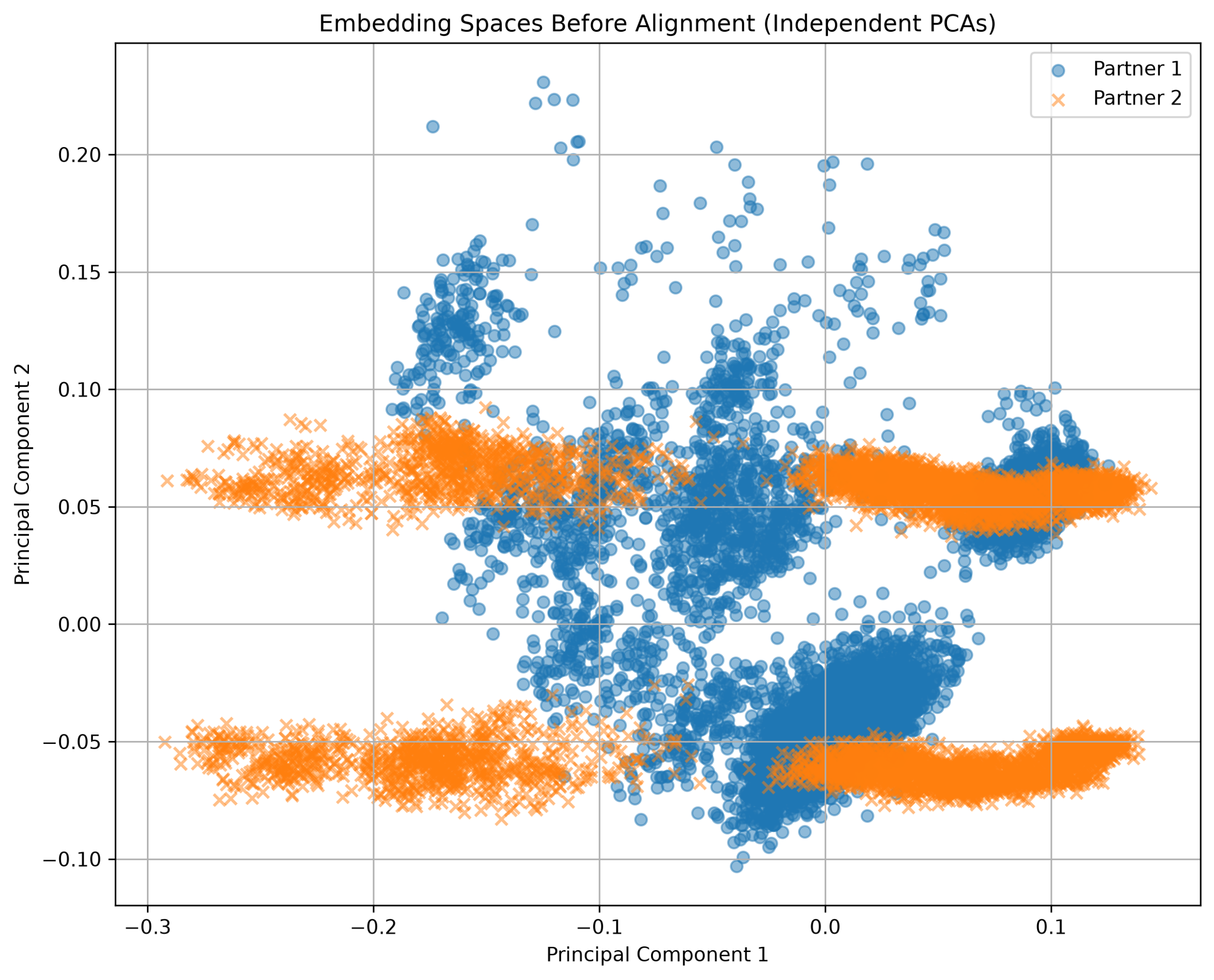
Such a difference in alignment is largely explained by the two models capturing different geometric structures in the data. This is reinforced by the plot below, which shows both embedding spaces pre-alignment projected down to 2 dimensions with independent PCA: Partner 2 exhibits 4 distinct clusters, whereas Partner 1 is more evenly spread. Because Orthogonal Procrustes is strictly an orthogonal rotation and reflection, it cannot alter intrinsic cluster topologies, preventing a perfect mapping.
Note: Interpretation of 2D Visualisations
The plot above is generated by projecting high-dimensional embedding spaces (64 to 1024 dimensions) down to 2 dimensions using PCA. Consequently, 2D proximity cannot be interpreted as a direct representation of geometric relationships in high-dimensional space. Furthermore, each partner’s embedding space is fitted with an independent PCA (2 components) and overlaid to illustrate intrinsic cluster shapes and structural distributions (cross-partner distances in this plot are not directly comparable).
The Best Non-Identical Embedding Combination (baai-base vs. gte-base)
In contrast, we look at the non-identical embedding combination which resulted in the best alignment performance: baai-base vs. gte-base.
Here, Recall@1 is 100%, demonstrating that the two embedding spaces can be mapped onto one another almost flawlessly with a simple orthogonal rotation.
This remarkable alignment is explained by their shared architectural lineage: both models were initialised from bert-base-uncased before being fine-tuned on separate corpora. Because downstream fine-tuning largely preserved the global coordinate structure, the two spaces remain related by a near-pure orthogonal rotation.
Further Results: Varying Anchor Availability
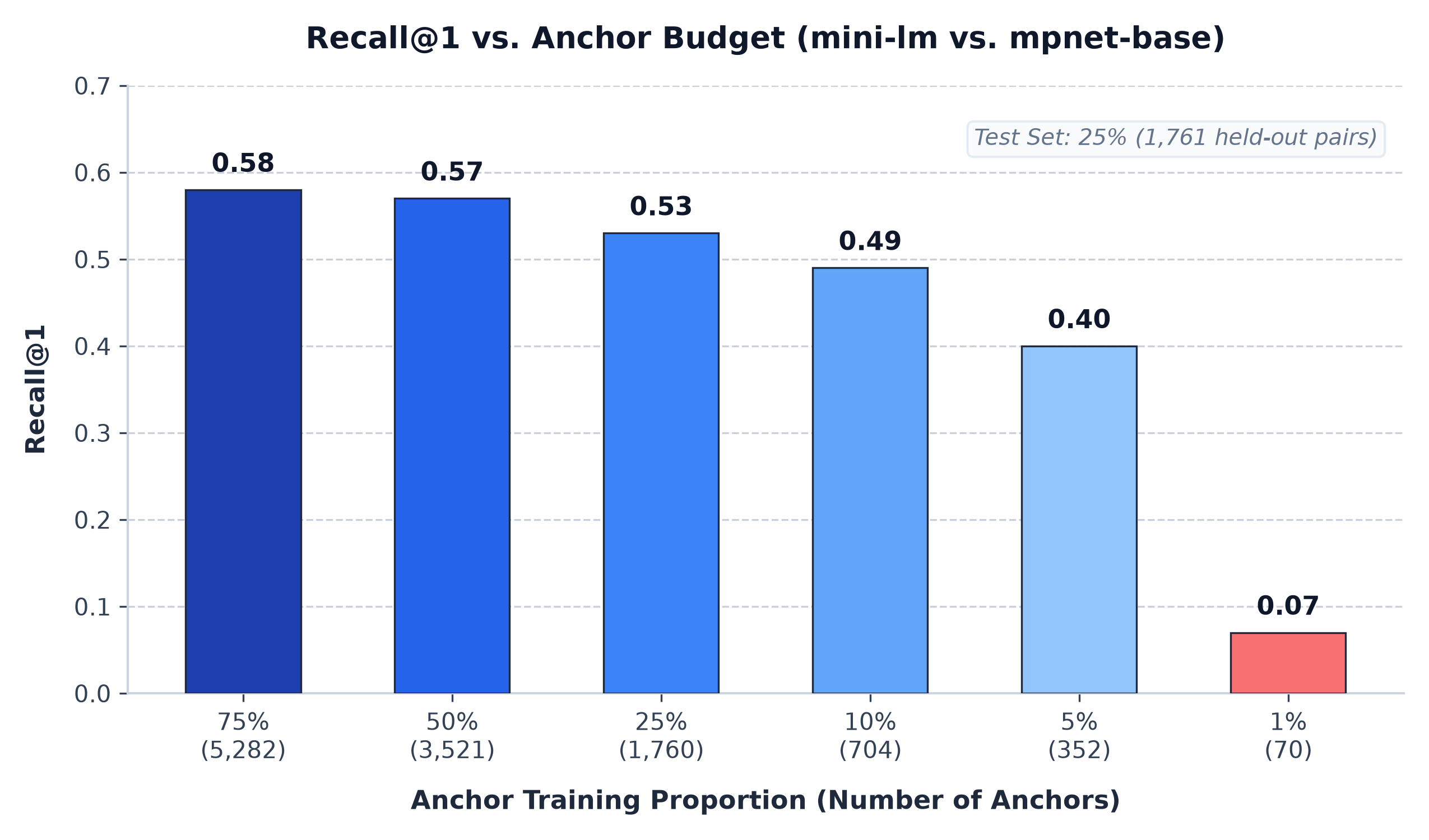
So far, our experiments have assumed access to 75% of the dataset as known anchor points. This is an optimistic assumption for real-world enterprise collaboration. We therefore systematically vary the proportion of training anchors provided to Procrustes across 75%, 50%, 25%, 10%, 5%, and 1% (corresponding to 5,282, 3,521, 1,760, 704, 352, and 70 training anchors, respectively), while holding the evaluation test set fixed at 25% (1,761 records). This gives us an indication of how much cooperation between companies is needed to achieve acceptable results.
From these experiments, we observe the following:
Same Encoder
As in the initial experiments, when both partners use the same embedding model, Recall@1 remains 100% regardless of the number of training anchors used. Even at the extreme limit of 1% training anchors (70 points), alignment is flawless because again both representations share identical underlying geometry, meaning Procrustes is unnecessary:
| P1 Embedding Model | P2 Embedding Model | Anchor Prop. | Anchors Used | Recall@1 | Recall@5 | Recall@10 | Recall@20 | Recall@30 | Recall@40 | Recall@50 |
|---|---|---|---|---|---|---|---|---|---|---|
baai-base |
baai-base |
0.75 | 5282 | 1.00 | 1.00 | 1.00 | 1.00 | 1.00 | 1.00 | 1.00 |
baai-base |
baai-base |
0.50 | 3521 | 1.00 | 1.00 | 1.00 | 1.00 | 1.00 | 1.00 | 1.00 |
baai-base |
baai-base |
0.25 | 1760 | 1.00 | 1.00 | 1.00 | 1.00 | 1.00 | 1.00 | 1.00 |
baai-base |
baai-base |
0.10 | 704 | 1.00 | 1.00 | 1.00 | 1.00 | 1.00 | 1.00 | 1.00 |
baai-base |
baai-base |
0.05 | 352 | 1.00 | 1.00 | 1.00 | 1.00 | 1.00 | 1.00 | 1.00 |
baai-base |
baai-base |
0.01 | 70 | 1.00 | 1.00 | 1.00 | 1.00 | 1.00 | 1.00 | 1.00 |
Top Performing Embedding Pairs
The top-performing non-identical pair in initial testing was baai-base and gte-base. As shown below, alignment performance remains high across all anchor budgets, highlighting the structural compatibility between these two spaces (both initialised from bert-base-uncased).
Performance only begins to soften at the extreme low-anchor regime of 1% training anchors (70 points), where Recall@1 is 98.7% and Recall@50 reaches 99.4%:
| P1 Embedding Model | P2 Embedding Model | Anchor Prop. | Anchors Used | Recall@1 | Recall@5 | Recall@10 | Recall@20 | Recall@30 | Recall@40 | Recall@50 |
|---|---|---|---|---|---|---|---|---|---|---|
baai-base |
gte-base |
0.75 | 5282 | 1.00 | 1.00 | 1.00 | 1.00 | 1.00 | 1.00 | 1.00 |
baai-base |
gte-base |
0.50 | 3521 | 1.00 | 1.00 | 1.00 | 1.00 | 1.00 | 1.00 | 1.00 |
baai-base |
gte-base |
0.25 | 1760 | 1.00 | 1.00 | 1.00 | 1.00 | 1.00 | 1.00 | 1.00 |
baai-base |
gte-base |
0.10 | 704 | 1.00 | 1.00 | 1.00 | 1.00 | 1.00 | 1.00 | 1.00 |
baai-base |
gte-base |
0.05 | 352 | 0.99 | 1.00 | 1.00 | 1.00 | 1.00 | 1.00 | 1.00 |
baai-base |
gte-base |
0.01 | 70 | 0.99 | 0.99 | 0.99 | 0.99 | 0.99 | 0.99 | 0.99 |
General Non-Identical Embedding Combinations
For the remaining non-identical embedding combinations, test anchor recall decreases as fewer training anchors are provided.
To illustrate these trends, the table below shows results for mini-lm vs. mpnet-base across all anchor training proportions:
| P1 Embedding Model | P2 Embedding Model | Anchor Prop. | Anchors Used | Recall@1 | Recall@5 | Recall@10 | Recall@20 | Recall@30 | Recall@40 | Recall@50 |
|---|---|---|---|---|---|---|---|---|---|---|
mini-lm |
mpnet-base |
0.75 | 5282 | 0.58 | 0.81 | 0.88 | 0.92 | 0.94 | 0.96 | 0.97 |
mini-lm |
mpnet-base |
0.50 | 3521 | 0.57 | 0.80 | 0.88 | 0.93 | 0.95 | 0.96 | 0.96 |
mini-lm |
mpnet-base |
0.25 | 1760 | 0.53 | 0.76 | 0.84 | 0.90 | 0.91 | 0.93 | 0.95 |
mini-lm |
mpnet-base |
0.10 | 704 | 0.49 | 0.72 | 0.81 | 0.88 | 0.91 | 0.92 | 0.93 |
mini-lm |
mpnet-base |
0.05 | 352 | 0.40 | 0.65 | 0.73 | 0.81 | 0.86 | 0.89 | 0.91 |
mini-lm |
mpnet-base |
0.01 | 70 | 0.07 | 0.20 | 0.29 | 0.37 | 0.44 | 0.49 | 0.55 |
Even for this lowest-performing combination, performance remains relatively strong down to moderate anchor budgets: Recall@20 exceeds 80% even when providing only 5% of anchors (352 points). Alignment degrades sharply only at the extreme 1% regime (70 anchors), where Recall@1 drops to 7% and Recall@50 to 55%, indicating that an under-sampled anchor set struggles to stabilise the global transformation against geometric drift.
Next Steps
- ▸Zero-Anchor Matching. Our immediate next step is examining methods to align spaces when no ground-truth anchors are shared. This will involve using dataset schemas and marginal distributions to construct synthetic anchors. Interestingly, as we observed diminished performance at the 1% anchor budget, synthetic anchor methods may also help stabilise low-anchor regimes.
- ▸Heterogeneous Cross-Domain Datasets. To make our approach applicable to real enterprise partnerships, we need to validate that alignment methods work when partner datasets feature different schemas and feature sets.
- ▸Specialised Tabular Encoders. In practice, enterprises will likely choose specialised architectures to encode tabular records (such as tabular AutoEncoders or self-supervised models) rather than sentence transformers. We will investigate whether specialised tabular encoders yield more consistent, robust geometric representations across different partners.