Author: Andreas Mastakouris

Abstract

Marketing teams often need to decide which campaign setup is worth testing before any budget is spent. The hard part is that performance does not depend on a single variable. It depends on the interaction between multiple factors, such as the brand, its audience, the campaign objective, the platform, the geography, and many other contextual signals.

This proof of concept from the Performance AI team at Open Intelligence (OI PoC) addresses this as a multimodal prediction and recommendation problem. We trained a single model that learns from historical campaign performance, predicts click-through rate (CTR), and uses the same learned embedding space to recommend campaign completions. The result is a system that can move from “what happened before?” to “what should we try next?” while staying grounded in real performance data.

This work builds on the earlier Campaign Performance Modelling Pod, which explored how AI can support campaign performance prediction using synthetic campaign data (see the Technical Report and Blog Post, respectively). The OI PoC analysis takes the next step by applying the same broader modelling agenda to observed/real performance data, trying to also examine both tasks of CTR prediction and recommendation in order to answer: given a partially specified campaign setup, what completion is most likely to perform well?

The prepared dataset contains 20,067 unique real campaign setups derived from 21,247,221 raw daily rows. The evaluation is designed as a warm-start compositional generalization problem: the model sees known modality values during training, but must generalize to unseen full combinations at test time. This is important because it mirrors the real planning use case more closely than simple row memorization.

In our evaluation, the model reached a test RMSE of 0.0151, MAE of 0.0052 and R2 of 0.6001 on unseen campaign combinations. For closed-vocabulary brand-fixed recommendations, the system achieved 76.2% positive precision@10 versus 50.2% for random selection from the same candidate pools, while reducing negative recommendations from 18.1% to 2.9%. For open-vocabulary recommendation, the strongest evidence appears in broader query settings where the model can still identify geometrically coherent completions that rank high relative to each brand’s historical CTR range.

1. Motivation

Campaign planning is highly combinatorial. A planner is not making one decision in isolation, but several interacting decisions at once: which audience to target, which campaign objective to optimize for, which platform to use, and which geography to prioritize for a given brand. Each of these choices can materially change the outcome, and the effect of any one decision depends on the others around it. In practice, that means the space of possible campaign setups grows much faster than the amount of historical evidence available to support them.

This follows naturally from the previous Campaign Performance Modelling work. The earlier synthetic-data analysis asked whether AI could help move campaign planning from intuition-led guesswork toward more systematic performance foresight. Here, we ask a complementary question: once real OI performance data is available, can we learn a performance-aware representation that supports both CTR prediction and recommendation?

This is exactly the gap OI PoC addresses. We want to help answer two related questions before budget is committed:

1. If a team is considering a particular campaign setup, what CTR should they expect?
2. If part of the setup is already fixed, what completion is most likely to perform well?

The challenge is that historical data is both rich and sparse at the same time. At the raw row level there is plenty of volume, but once performance is aggregated into distinct campaign setups, only a small fraction of the theoretically possible combinations has ever been observed. A useful model therefore cannot depend on exact lookup or memorization. It needs to learn reusable structure from known examples and then transfer that structure to unseen combinations.

This creates several practical modelling challenges:

1. Prediction models can accidentally memorize historical rows instead of learning reusable structure.
2. Recommendation systems can look accurate when the available candidate pool is already easy, even if the model is not adding much ranking value.
3. Performance labels are not globally comparable across brands, because some brands naturally operate at different CTR ranges than others.
4. Recommendation quality depends not just on whether a setup looks broadly similar to past positives, but on whether its internal combination of brand, audience, objective, platform and geography is coherent.

The goal of OI PoC was to build a model that could generalize across known campaign ingredients in new configurations. This is a warm-start compositional generalization problem: the model has usually seen the individual ingredients before, but not the exact recipe. That is why the project combines CTR prediction and recommendation in a shared multimodal framework. The prediction side estimates likely performance for unseen setups, while the recommendation side uses the same learned representation to identify strong or plausibly strong completions for partially specified queries.

2. Dataset

The raw source dataset contained 21,247,221 daily campaign rows. After aggregation by campaign setup and filtering low-signal rows, this reduced to 20,067 unique learnable combinations. Furthermore, brand values were anonymized before being used as modelling inputs. This preserves the ability to learn brand-specific performance behaviour while keeping the modelling dataset separated from directly identifiable brands.

The five campaign modalities and their coverage are summarized in Table 1:

The train, validation and test split used 17,056 training rows, 1,505 validation rows and 1,506 test rows. The test set was designed to avoid exact-combination leakage.

The split diagnostics are reported in Table 2:

This means the evaluation is not a pure cold-start task. It is a test of whether the model can recombine known entities into unseen campaign setups.

3. Why CTR Needed Brand-Relative Labels

Click-through rate (CTR) serves as our example performance metric—a practical starting point given the available data. We use it across the dataset, including campaigns with objectives other than clicks, to explore whether the approach can support prediction and recommendation. The positive, neutral and negative labels therefore describe brand-relative CTR, not success against each campaign’s stated objective. Stronger click-through performance does not necessarily indicate stronger awareness, engagement or video-view outcomes. The next step is to extend the approach to available metrics better suited to those objectives.

CTR distribution statistics are shown in Table 3, proving that CTR was highly skewed:

A global definition of “positive” campaign performance would over-favour brands with naturally higher CTR and penalise brands with lower typical CTR. Instead, each brand’s own CTR distribution was split into rank-based thirds: negative, neutral and positive.

This created labels that mean “good for this brand”, rather than “high CTR globally”. The anonymized brand identifiers are still consistent across rows, which means the model can learn within-brand CTR patterns without needing access to the original brand names.

The final label distribution is reported in Table 4:

Rank-based splitting was used because many brands had zero-heavy CTR distributions. Standard quantile thresholds often collapsed to the same value, while rank-based labels preserved useful within-brand ordering.

4. Model Approach

OI PoC uses one shared model for both prediction and recommendation.

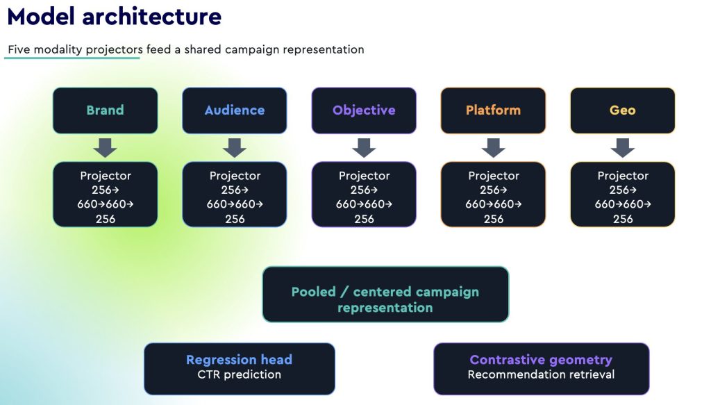
Each modality starts from a 256-dimensional embedding and passes through its own projector:

• brand projector
• audience projector
• objective projector
• platform projector
• geography projector

The projected modality embeddings are pooled into a shared campaign representation. From there, the model optimizes two signals:

• a regression head predicts transformed CTR;
• a centered contrastive objective shapes the embedding geometry so that positive, neutral and negative campaign setups become easier to retrieve and rank.

The shared model architecture is illustrated in Figure 1:

The centered contrastive objective is important because it encodes a more useful recommendation bias than a standard label-only contrastive loss. In this setting, we do not simply want all positive examples to collapse toward one another in the embedding space. Two campaign setups can both be labelled positive while being strategically very different in terms of brand, audience, objective, platform and geography. Forcing all positives to become globally similar would risk bringing together irrelevant campaign setups that happen to share the same final label but not the same internal structure.

Instead, the centered loss focuses on intra-sample consistency. For each projected modality embedding, the model compares it against the center formed by the other modalities within the same campaign setup. This encourages the representation to answer a more precise question: do the parts of this setup belong together in a performance-aware way? Positive tuples should exhibit stronger internal agreement, neutral tuples should sit closer to an intermediate structure, and negative tuples should show weaker alignment. That is much closer to the actual recommendation task, where the model needs to judge whether a partially specified setup can be completed coherently rather than whether it merely resembles some broad global “positive” cloud.

This design also makes the loss batch-sensitive in a useful way. The implementation weights modality contributions using both global and batch-level information. Global weighting reflects the overall cardinality of each modality vocabulary, while batch weighting reflects the effective diversity of modality values present in the current batch. In practice, this helps prevent the contrastive term from over-responding either to globally large modalities such as audience or to accidentally repetitive mini-batches where one modality has very little variation. The current implementation uses gamma_global = 0.5 and gamma_batch = 0.5, which gives a balanced influence to long-run dataset structure and local batch composition.

The centered loss is also deliberately moderated relative to the CTR objective. In training, the total loss combines Huber regression with the centered contrastive term using LAMBDA_CENTERED = 0.05, plus a small norm penalty inside the contrastive component. This keeps CTR prediction as the dominant optimization target while still giving the embedding space enough geometric structure to support retrieval and reranking. The result is a representation that is not purely semantic and not purely regressive: it is shaped to preserve campaign-setup compatibility in a way that is directly useful for recommendation.

This design keeps deployment simple: one model artifact, one embedding space and one monitoring surface. It also makes the recommendation layer performance-aware rather than purely semantic.

5. Evaluation Design

The evaluation focused on three questions:

1. Can the model predict CTR for unseen campaign combinations?
2. Can the learned representation identify stronger recommendations than random selection from the same candidate pool?
3. Can the model propose new combinations in open vocabulary settings without simply replaying historical rows?

For recommendations, the system uses a two-stage retrieve-then-rerank pipeline, as summarized in Table 5:

This is important operationally because the embedding space provides a fast candidate filter, while the regression head gives the final ranking signal.

6. Regression Results

As reported in Table 6, on the 1,506-row test set the model captured a meaningful share of CTR variance for unseen combinations:

The model is useful but conservative in high-CTR slices. For LINK_CLICKS, the actual average CTR was 0.02370 while the predicted average CTR was 0.01938, a bias of -0.00432. This is expected given the heavy-tailed target distribution and should be monitored before production use.

Permutation diagnostics are shown in Table 7, demonstrating that objective and platform were the strongest regression drivers:

The geography result is likely influenced by the dataset composition, where the prepared rows are heavily UK-centered.

7. Closed-Vocabulary Recommendation Results

Closed-vocabulary recommendations are completions drawn from rows already present in the historical dataset. This lets us evaluate recommendation quality against known labels.

In practical terms, “closed” means the recommender is choosing from campaign setups that have already been observed historically, rather than inventing entirely new combinations. That makes this the most directly measurable recommendation setting: every retrieved completion can be checked against an existing brand-relative label, so we know whether the model is surfacing historically positive, neutral or negative outcomes. Closed-vocabulary evaluation is therefore the clearest test of ranking quality. If the model is genuinely useful, it should place more positive combinations near the top of the list and push negative combinations down, even when the available candidate pool is mixed.

We group recommendation queries by how much of the campaign setup is already fixed. “Brand only” fixes the brand and leaves audience, objective, platform and geography open for recommendation. “Brand + 1” fixes the brand plus one of those four ingredients; “Brand + 2” fixes the brand plus two; and “Brand + 3” fixes the brand plus three. For example, a query with a fixed brand and objective is a “Brand + 1” query: the model recommends the remaining audience, platform and geography.

Overall closed-vocabulary results are reported in Table 8. Across 57 valid evaluated brand-fixed queries, OI PoC achieved:

The model produced a 1.92x positive lift versus random selection and reduced negative recommendations by 15.1 percentage points.

Results by query type are presented in Table 9. The strongest result came from broader brand-fixed queries:

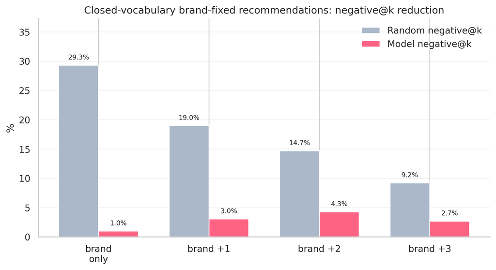
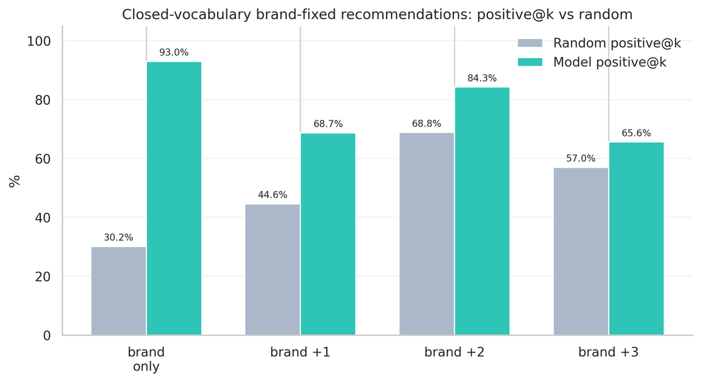
Figure 2 shows the positive recommendation rate by query type, while Figure 3 shows the corresponding negative recommendation rate. The former demonstrates how often the top recommendations fall into the historically positive class for each query type. This is the most intuitive measure of recommendation value: higher is better, because it means the model succeeds in surfacing combinations that were historically strong for the given brand. The latter depicts the opposite side of the same story. Lower is better, because it means the recommender is avoiding combinations that were historically weak.

These plots are important because raw precision alone can be misleading if the candidate pool is already easy. That is why the comparison against random selection from the same candidate pool matters so much. The model is not just scoring well because it is choosing among already strong options. In brand-only queries, the historical candidate pool contains only about 30.2% positives, yet the recommender raises positive precision@10 to 93.0% and cuts negatives from 29.3% to 1.0%. Brand + 1 remains very strong, with 44.6% candidate positives rising to 68.7% positive@10 and negatives falling from 19.0% to 3.0%. Brand + 2 is still strong, lifting positives from 68.8% to 84.3% and lowering negatives from 14.7% to 4.3%.

Brand + 3 needs a more careful reading. On the surface, 65.6% positive@10 and 2.7% negative@10 still look solid. But the candidate pool for this case is already extremely favourable, with 57.0% positives and only 9.2% negatives before the model ranks anything. In other words, once four parts of the setup are already fixed, there is often very little ranking difficulty left. That is why the lift versus random is close to flat in this setting. The model is still producing sensible recommendations, but the closed-vocabulary evidence no longer shows a strong ranking advantage over the baseline.

The interpretation is therefore more nuanced than simply saying “the model works everywhere.” Closed-vocabulary results show clear ranking value when the query leaves enough room for the model to discriminate among many possible completions. That is most visible in brand-only, brand + 1 and still present in brand + 2 queries, and much less convincing in brand + 3 where the space is already heavily constrained. This is exactly the kind of pattern we would hope to see from a recommender that is useful in realistic planning scenarios rather than only in highly filtered cases.

8. Open-Vocabulary Recommendation Results

Open-vocabulary recommendations generate combinations that are mostly not present in the historical dataset. This is the more interesting planning use case, but also the harder one to validate offline.

Because most open-vocabulary recommendations are unknown historically, the evaluation relies on geometric diagnostics and predicted CTR relative to each brand’s historical distribution.

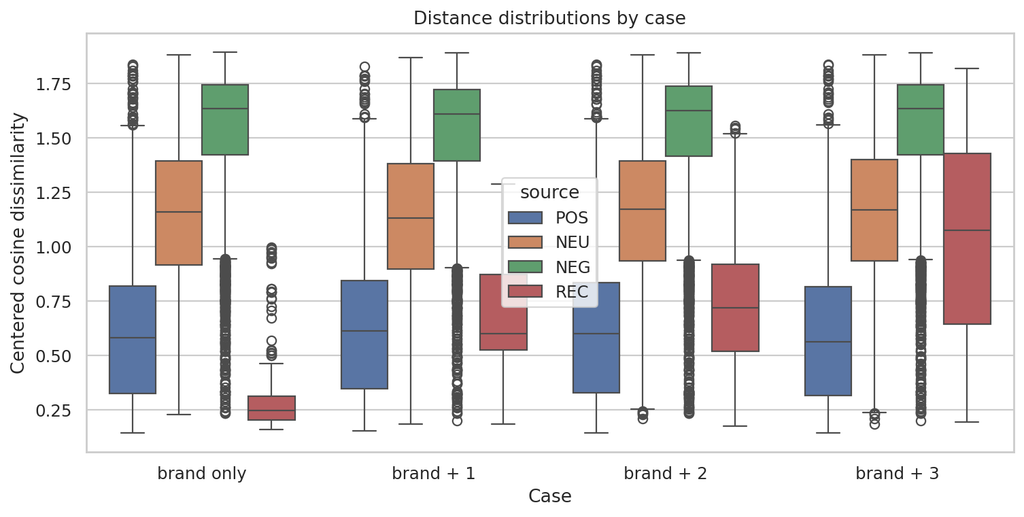
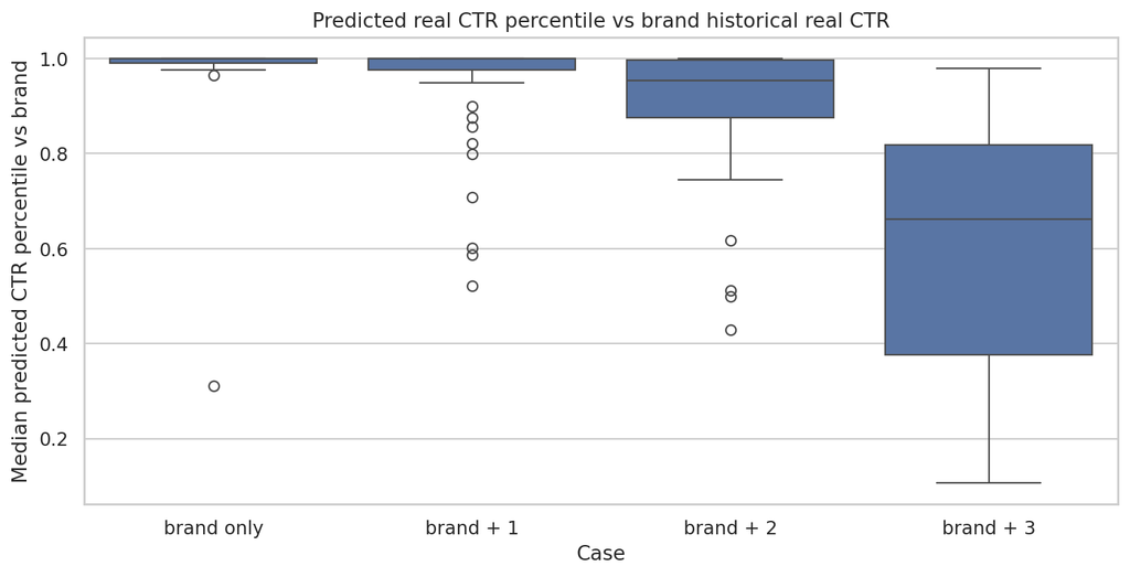
Two diagnostics are especially useful here. The first is centered cosine dissimilarity, which measures how well a recommended completion fits the learned geometry of a query. Lower dissimilarity means the retrieved combination sits closer to the model’s positive reference structure; higher dissimilarity suggests a weaker or more ambiguous fit. The second is predicted CTR percentile versus brand history, which asks where the model’s predicted CTR for a recommendation sits relative to that brand’s own historical CTR distribution. A percentile near 1.0 means the recommendation is predicted to perform near the top end of what that brand has historically achieved, while a percentile closer to 0.5 means the recommendation looks more typical than exceptional.

Overall open-vocabulary diagnostics are summarized in Table 10:

As depicted in Figure 4, the centered cosine dissimilarity plot shows that the model is most confident in broad recommendation settings. Brand-only queries have the strongest geometric fit, followed by brand + 1 and brand + 2 queries. This is consistent with the retrieval results: when the query leaves enough freedom for the model to search the space, the learned geometry can still find combinations that resemble historically positive structures. Brand + 3 behaves differently, with substantially weaker positive-distribution alignment and a higher negative-distribution rate. This suggests that once the query becomes too constrained, the geometry has much less room to identify clearly superior completions.

The CTR percentile plot tells a complementary story (see Figure 5). For brand-only recommendations, the mean predicted CTR lands around the 98.1st percentile of the brand’s historical distribution. Brand + 1 remains similarly strong at 94.9%, and brand + 2 still sits high at 91.2%. These are not just ‘acceptable’ completions; they are recommendations whose predicted CTR places them near the upper end of each brand’s historical range. Brand + 3 drops to roughly the 64.7th percentile, which is still above median, but much less distinctive. In other words, the model still finds plausible completions in this more constrained setting, but it is no longer consistently surfacing outcomes that look clearly elite for the brand.

Taken together, the two plots support the same interpretation. The open-vocabulary recommender is most credible when it has enough flexibility to discover new completions rather than simply fill in one missing slot in an already highly specified setup. In broad and moderately constrained contexts, the recommended combinations both align strongly with the positive geometry of the learned space and score highly against the brand’s own historical CTR range. In heavily constrained contexts, the model can still produce sensible outputs, but the diagnostic strength is noticeably weaker and the case for production use becomes more cautious.

Low known@10 is expected and desirable in this setting: it means the recommender is proposing new combinations rather than simply replaying historical rows. The overall known@10 rate is only 5.0%, confirming that most recommended combinations are genuinely new relative to the historical dataset.

Overall, the strongest open-vocabulary evidence appears for brand-only, brand + 1 and brand + 2 queries. Brand + 3 degrades materially because the query is already highly constrained and leaves less room for the model to improve the completion.

9. What This Enables

OI PoC turns historical campaign data into a planning tool with three practical uses:

1. CTR prediction for unseen combinations of known campaign entities.
2. Brand-relative recommendation, where “positive” means strong for that brand rather than globally high CTR.
3. Discovery of new campaign completions that are plausible in the learned performance-aware embedding space.

The most defensible claim from the current results is:

Among sufficiently supported queries, the model improves positive recommendation rate and sharply reduces negatives versus random selection, especially for brand-only, brand + 1 and brand + 2 recommendation contexts.

What’s next?

There are several directions we’re excited to explore from here. One is understanding when the model is confident enough in a recommendation to make it useful, combining signals such as retrieval distance, predicted CTR and the diversity of the candidate pool.

We’re also interested in making recommendations easier to interpret: which modalities contribute most to predicted CTR, and what makes a particular campaign completion rank highly?

Another direction is improving calibration across high-CTR segments and objectives such as LINK_CLICKS, while continuing to validate open-vocabulary recommendations with expert review.

Ultimately, the most interesting question is how these recommendations perform beyond offline evaluation. A controlled online experiment comparing model-recommended campaign completions with existing planning approaches would be a natural next step.

There’s more to explore here — stay tuned.