Author: Anastasios Tsourtis

  • LLM Routing with Jev: Accuracy, Latency, and Cost

    Large language model routing aims to reduce inference cost and latency by matching each request to an appropriate model tier without materially degrading answer quality. This study compares three request-classification strategies: Gemini 2.5 Flash Lite, TypeSafe’s Jev, and LiteLLM’s default heuristic using simple, medium, and reasoning models. We evaluate each strategy on samples from four public datasets, measuring answer accuracy, classification and response latency, classification and response cost, and model-selection patterns. Our goal was to investigate whether routers can choose the right level of “brainpower” for each question instead of always relying on the most powerful and expensive model. Jev offered the strongest overall balance, making routing decisions faster and more cost efficient than Gemini while delivering broadly comparable accuracy. The results show that smarter routing can make AI applications faster and more affordable, although the best approach will depend on an organisation’s accuracy needs, budget, and data-privacy requirements.

    Motivation – Allocating cognition at the request-level

    In our previous article, Cost-Aware LLM Request Routing: From Tokenomics to Dynamic Cognitive Allocation [1], we examined why applications should allocate model capacity according to the requirements of each request. Model providers now offer LLMs with different levels of capability, latency, and cost. Sending every request to the most capable model can consume more time and money than the task requires. Sending every request to the cheapest model creates the opposite risk: difficult tasks may receive answers from a model that lacks the required reasoning capability.

    An LLM router selects a model for each incoming request. In a fixed configuration, a developer chooses the model in advance, and every request follows the same route. Dynamic routing removes this assumption. The application has no a priori knowledge of which model a request requires, so the router classifies the request and assigns it to a capability tier, such as simple, medium, or reasoning. The router must balance three requirements:

    • Accuracy measures whether the selected model answers the request correctly.
    • Classification latency measures how much time the classification step adds before the selected model begins processing the request. Response latency measures the time required for an autoregressive model (LLM) to provide a full answer where reasoning models take longer.
    • Cost includes both the classification step and the model that produces the answer.

    Routing therefore introduces an additional step before the answer is generated. This step adds classification cost and latency, but it can reduce response cost and response latency by directing suitable requests to less expensive and faster models. A useful router must produce enough savings at the response stage to justify its classification overhead, without causing an unacceptable loss in answer accuracy.

    In this article, we test three classification components for an LLM router: a lightweight LLM, Jev, and a keyword-based heuristic classifier. We compare their answer accuracy, classification latency, classification cost, response cost, and end-to-end response latency with fixed model selection.

    Jev: Structured Decisions Without Text Generation

    Jev [2] is TypeSafe’s first System One model. The name draws on the distinction between fast, intuitive System 1 thinking and slower, deliberate System 2 reasoning, popularised by Daniel Kahneman in Thinking, Fast and Slow [3]. In this context, System One refers to focused judgments that do not require a written explanation. Jev applies this approach to natural-language input and returns structured values that software can use directly.

    This design differs from that of a conventional large language model. An LLM generates text one token at a time, even when an application only needs a category or score. The application must then parse and validate the generated text before it can act on the result. Jev does not generate a written response. It evaluates a defined question against the supplied state, which contains the request and any context needed to classify it, and returns an answer in a format specified by the application.

    Jev exposes classification through question types called primitives. For LLM routing, the relevant primitive is Choice, which selects one option from a fixed set. In our router, the options are SIMPLE, MEDIUM, and REASONING. Each option represents a model tier with a different balance of capability, latency, and cost. Jev evaluates the incoming request against these options, and the application sends the request to the model assigned to the selected tier.

    A Choice response contains three parts:

    • choice identifies the selected model tier.
    • probabilities reports the probability assigned to every available tier.
    • confidence describes how strongly the probability distribution favours one option.

    The distinction between probabilities and confidence matters when a request lies near the boundary between two tiers. A router can use a high-confidence classification directly and route a low-confidence request to a more capable model. Confidence does not guarantee that an individual decision is correct. TypeSafe describes Jev’s probabilities as calibrated across groups of predictions, meaning that higher probabilities should correspond to higher observed accuracy when results are evaluated over many requests.⁠

    Jev’s suitability can be considered against the routing requirements introduced in the motivation:

    • For accuracy, Jev’s probabilities and confidence expose uncertainty about the selected tier, while Choice ensures that the output is one of the permitted routing options. Whether those selections preserve answer accuracy must be determined from the responses produced by the selected models.
    • For latency, Jev adds the time required to classify the request before the selected model can answer it. The relevant measurements are therefore the classification latency and the end-to-end response latency.
    • For cost, Jev incurs a classification cost and influences the response cost through the model tier it selects. A lower classification cost does not by itself imply a lower combined cost; the classification and response costs must be considered together.

    These properties explain why Jev is a plausible classification solution, but they do not establish whether it selects the appropriate tier or improves the balance between accuracy, latency, and cost. Our experimental evaluation using LiteLLM as the proxy service [4] tests this proposition. It begins with fixed-model baselines and then compares three routing strategies: an LLM classifier, Jev, and a keyword-based heuristic classifier.

    Experimental evaluation over multiple routing strategies

    Datasets

    We evaluate the routing strategies on four evaluation sets with different reasoning requirements. The sets are derived from PIQA, WorldSense, and RouterBench. PIQA and WorldSense are available through Inspect Evals [5, 6, 8], while RouterBench combines questions from several established benchmarks [7].

    The full evaluation sets contain between 1,838 and 40,176 questions. Each experimental condition uses a sample of 100 questions from each set. Table 1 summarises the available sample size, answer format, included content, and reasoning level assigned in our experimental design.

    Evaluation set Available samples Answer choices Included content Reasoning
    PIQA [5] 1,838 2 Binary question answering Easy
    WorldSense, all categories [6] 40,176 2–3 All WorldSense categories, including questions that may be impossible to decide Hard
    WorldSense, completion and normal [6] 3,348 2–3 completion problems and normal categories Hard
    RouterBench subset [7] 26,816 2–4 MMLU, HellaSwag, WinoGrande, and ARC-Challenge Medium–Hard

    Table 1. Evaluation sets used in the routing experiments. Each experiment uses 100 sampled questions from each set.

    Representative questions

    The following examples illustrate the answer formats used in PIQA and WorldSense.

    PIQA example

    Input: Make outdoor pillow.
    Choices: A: Blow into tin can and tie with rubber band. B: Blow into trash bag and tie with rubber band.
    Target: B

    WorldSense example

    Input: There are three people of different heights in a room: Patricia is taller than Grace, and Patricia is taller than Robert. Choose one of the following alternatives: 1. Robert is taller than Grace. 2. Robert is shorter than Grace. 3. It is impossible to decide.
    Choices: 1, 2, 3
    Target: 3

    The harder WorldSense subset contains two categories:

    • completion problems asks which statement follows from a description and includes cases where the answer cannot be determined.
    • normal contains questions that the evaluation describes as requiring a world model to solve.

    RouterBench contains multiple-choice questions drawn from MMLU, HellaSwag, WinoGrande, and ARC-Challenge. The questions have two, three, or four possible answers.

    Prompt format

    We convert every question to the same prompt format so that responses can be parsed and evaluated consistently:

    prompt = (
    f"Input: {input_text}\n"
    f"Choices: {choices}\n"
    "Which choice is correct? "
    "DO NOT try to explain your answer."
    )

    We instruct each model to return only the selected option so that answers can be parsed and evaluated consistently. This instruction limits the visible response, but provider-reported reasoning tokens, where applicable, remain part of the model usage and cost.

    Before comparing the routing strategies, we establish fixed-model baselines to measure how the simple and reasoning models perform on these evaluation sets.

    Baseline: pinned models

    We first establish two fixed-model baselines. In each baseline, we pin one model in the LiteLLM proxy and use that model for every request. There is no classification step and no dynamic selection between models.

    The first baseline uses gemini-2.5-flash-lite, which represents the simple tier. The second uses gemini-2.5-pro, which represents the reasoning tier. Both models come from the same provider and model family, limiting variation unrelated to the choice of model.

    For each evaluation set, we randomly sample 100 questions and measure answer accuracy and the total wall-clock time required to process them. Requests are submitted with a concurrency of five.

    A configuration consists of one model evaluated on one evaluation set. We evaluate each configuration over three independent runs. Across these runs, answer accuracy varies by approximately two percentage points, while wall-clock time varies by approximately 5%. Provider load is not controlled and may contribute to the observed timing variation.

    Table 2. Observed answer accuracy and total evaluation time for the two fixed-model baselines. Each configuration uses 100 questions and a concurrency of five. Accuracy varies by approximately two percentage points across three independent runs, while total evaluation time varies by approximately 5%.
    Evaluation set gemini-2.5-flash-lite
    accuracy
    gemini-2.5-flash-lite
    total evaluation time
    gemini-2.5-pro
    accuracy
    gemini-2.5-pro
    total evaluation time
    PIQA 87% 13.2 s 96% 170 s
    RouterBench 79% 13.5 s 89% 193 s
    WorldSense 44% 14.8 s 89% 190 s
    WorldSense, completion and normal 63% 13.4 s 98% 190 s

    Table 2 shows that gemini-2.5-pro achieves higher observed accuracy than gemini-2.5-flash-lite on all four evaluation sets. The observed difference is 9 percentage points on PIQA, 10 on RouterBench, 45 on WorldSense, and 35 on WorldSense completion and normal. These differences should be read alongside the run-to-run variation reported above.

    The higher observed accuracy is accompanied by a substantial increase in processing time. gemini-2.5-flash-lite processes each evaluation set in 13.2 to 14.8 seconds, whereas gemini-2.5-pro, requires 170 to 193 seconds.

    These fixed-model results provide reference points for the routing experiments. Sending more requests to gemini-2.5-pro may preserve or improve answer accuracy, but it also increases response latency and cost. Sending more requests to gemini-2.5-flash-lite reduces response latency and cost, but may reduce accuracy. The routing experiments test whether a classifier can manage this trade-off by selecting among the available model tiers for each request.

    Smart routing, option 1: Gemini classifier

    The first routing strategy uses a lightweight language model as the classifier. For each request, the classifier selects one of three available models. This is part of the LiteLLM configuration file:

    tiers:

    SIMPLE: gemini-2.5-flash-lite

    MEDIUM: gemini-2.5-flash

    REASONING: gemini-2.5-pro

    classifier_llm_config:
    model: gemini-2.5-flash-lite

    The classifier uses gemini-2.5-flash-lite to evaluate the input and select a model. LiteLLM then sends the original request to the selected model.

    The model selections are outputs of the classifier, not ground-truth labels. The experiments therefore do not measure whether the classifier selects an objectively correct model for each question. Instead, we evaluate the resulting system using final-answer accuracy, latency, cost, and the distribution of requests across the three models.

    Figure 1 shows how the Gemini classifier distributes the 100 questions from each evaluation set. The panels follow the reasoning order established in Table 1: PIQA, RouterBench, WorldSense, and WorldSense completion and normal.
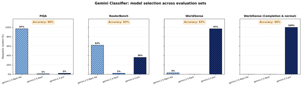
    Model selection by the Gemini classifier across the four evaluation sets, ordered by their assigned reasoning difficulty. Answer accuracy is shown inside each panel. The classifier moves from predominantly selecting gemini-2.5-flash-lite for PIQA to predominantly selecting gemini-2.5-pro for the two hard WorldSense sets, while RouterBench produces a mixture of the simple and reasoning models.

    For PIQA, the classifier routes 97 of the 100 questions to gemini-2.5-flash-lite, 1 to gemini-2.5-flash, and 2 to gemini-2.5-pro. The resulting system answers 90 questions correctly. For RouterBench it produces a more varied distribution. The classifier routes 62 questions to gemini-2.5-flash-lite, 2 to gemini-2.5-flash, and 36 to gemini-2.5-pro. The resulting system answers 83 questions correctly. The distribution changes for the two hard WorldSense sets. The classifier routes 97 WorldSense questions to gemini-2.5-pro and all 100 questions from WorldSense completion and normal to that model. The resulting system answers 93 and 99 questions correctly, respectively.

    Table 3 reports answer accuracy, model selection, classification cost and latency, response cost and latency, and output-token use. Classification measurements cover the routing decision, while response measurements cover the routed request and the selected model’s response. Cost, latency, and token measurements are reported per request. Total evaluation time is the wall-clock time required to process all 100 questions.

    Metric
    PIQA
    RouterBench
    WorldSense
    WorldSense, completion and normal
    Accuracy
    90%
    83%
    93%
    99%
    Total evaluation time
    61.5 s
    104.9 s
    186.2 s
    209.9 s
    Model selection [gemini-2.5-flash-lite,
    gemini-2.5-flash,
    gemini-2.5-pro]
    [97%, 1%, 2%]
    [62%, 2%, 36%]
    [3%, 0%, 97%]
    [0%, 0%, 100%]
    Classification cost ($/request)
    Mean ± standard deviation
    (range)
    4.22e-05 ± 3.58e-06
    (3.69e-05 to 5.98e-05)
    5.10e-05 ± 9.19e-06
    (3.92e-05 to 7.43e-05)
    4.47e-05 ± 1.79e-06
    (4.17e-05 to 5.07e-05)
    4.67e-05 ± 1.72e-06
    (4.30e-05 to 5.09e-05)
    Response cost ($/request)
    Mean ± standard deviation
    (range)
    1.20e-04 ± 7.40e-04
    (5.50e-06 to 5.60e-03)
    4.50e-03 ± 7.00e-03
    (7.40e-06 to 3.40e-02)
    1.00e-02 ± 1.20e-02
    (1.10e-05 to 1.20e-01)
    1.20e-02 ± 3.00e-03
    (5.00e-03 to 2.60e-02)
    Response latency (ms)
    Mean ± standard deviation
    (range)
    1,307 ± 633
    (1,039 to 5,587)
    4,959 ± 5,779
    (1,026 to 28,201)
    8,926 ± 9,167
    (1,133 to 90,427)
    10,135 ± 2,416
    (5,564 to 20,388)
    Classification latency (ms)
    Mean ± standard deviation
    (range)
    666 ± 180
    (493 to 1,612)
    643 ± 74
    (564 to 1,006)
    644 ± 65
    (535 to 877)
    720 ± 81
    (594 to 1,175)
    Output tokens
    Mean ± standard deviation
    (range)
    27 ± 124
    (1 to 834)
    462 ± 704
    (1 to 3,385)
    942 ± 499
    (1 to 3,773)
    1,216 ± 348
    (609 to 2,402)

    Table 3. Performance of the Gemini classifier across four evaluation sets, using 100 questions from each set. Total evaluation time refers to the complete evaluation run. All other cost, latency, and token measurements are reported per request.

    Table 3 shows that mean classification latency remains between 643 and 720 ms across the four evaluation sets. Mean classification cost similarly remains between $4.22e-05 and $5.10e-05 per request. The classification stage therefore introduces a relatively consistent measured overhead across these experiments.

    Response latency and cost vary more substantially. PIQA has a mean response latency of 1,307 ms and a mean response cost of $1.20e-04 per request. These values increase to 4,959 ms and $0.0045 on RouterBench, 8,926 ms and $0.010 on WorldSense, and 10,135 ms and $0.012 on WorldSense completion and normal.

    This variation accompanies the change in model selection shown in Figure 1. The Gemini classifier predominantly selects gemini-2.5-flash-lite for PIQA but predominantly selects gemini-2.5-pro for the two WorldSense sets. RouterBench falls between these cases, with requests divided mainly between the simple and reasoning models.

    The output-token measurements follow a similar pattern. PIQA has a mean of 27 output tokens per request, compared with 462 for RouterBench, 942 for WorldSense, and 1,216 for WorldSense completion and normal. These are provider-reported usage measurements and should not be interpreted as visible answer length. The prompt instructs each model to return only the selected option, but provider-reported reasoning tokens, where applicable, remain part of model usage and cost.

    The Gemini classifier provides a model-based reference for the remaining experiments. We next retain the same three downstream models and replace the Gemini classification step with Jev. This allows us to compare the two classifiers without changing the models available to the router.

    Smart routing, option 2: Jev classifier

    We next replace the Gemini classifier with Jev while retaining the same three downstream models. This allows us to compare the two classifiers without changing the models available to the router.

    The experiments use Jev version 1.13.0, integrated through LiteLLM version 1.103.0rc01. The relevant LiteLLM configuration is:

    tiers:

    SIMPLE: gemini-2.5-flash-lite

    MEDIUM: gemini-2.5-flash

    REASONING: gemini-2.5-pro

    classifier_type:
    model: jev

    jev_classifier_config:

    model: jev-latest

    Figure 2 shows how Jev distributes the 100 questions from each evaluation set. As in Figure 1, the panels are ordered by their assigned reasoning difficulty: PIQA, RouterBench, WorldSense, and WorldSense completion and normal.
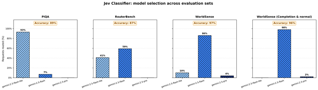
    Model selection by the Jev classifier across the four evaluation sets, ordered by their assigned reasoning difficulty. Answer accuracy is shown inside each panel. Jev moves from predominantly selecting gemini-2.5-flash-lite for PIQA to predominantly selecting gemini-2.5-flash for the two hard WorldSense sets, while selecting gemini-2.5-pro for only 6 questions across all four experiments.

    For PIQA, Jev routes 93 of the 100 questions to gemini-2.5-flash-lite and 7 to gemini-2.5-flash. The resulting system answers 89 questions correctly. For RouterBench, Jev divides the questions between the simple and medium models. It routes 41 questions to gemini-2.5-flash-lite and 59 to gemini-2.5-flash, producing 87 correct answers. For WorldSense, Jev routes 10 questions to gemini-2.5-flash-lite, 86 to gemini-2.5-flash, and 4 to gemini-2.5-pro. For WorldSense completion and normal, it routes 98 questions to gemini-2.5-flash and 2 to gemini-2.5-pro. The resulting system answers 97 and 96 questions correctly, respectively.

    Table 4 reports the complete Jev results. As in Table 3, total evaluation time covers the complete run of 100 questions. Cost, latency, token, and confidence measurements are reported per request.

    Metric
    PIQA
    RouterBench
    WorldSense
    WorldSense, completion and normal
    Accuracy
    89%
    87%
    97%
    96%
    Total evaluation time
    23.7 s
    70.4 s
    78.6 s
    132.1 s
    Model selection [gemini-2.5-flash-lite,
    gemini-2.5-flash,
    gemini-2.5-pro]
    [93%, 7%, 0%]
    [41%, 59%, 0%]
    [10%, 86%, 4%]
    [0%, 98%, 2%]
    Classification cost ($/request)
    Mean ± standard deviation
    (range)
    2.15e-05 ± 1.50e-06
    (1.96e-05 to 2.89e-05)
    2.45e-05 ± 4.88e-06
    (0 to 3.23e-05)
    2.23e-05 ± 7.20e-07
    (2.10e-05 to 2.40e-05)
    2.30e-05 ± 7.50e-07
    (2.14e-05 to 2.46e-05)
    Response cost ($/request)
    Mean ± standard deviation
    (range)
    7.42e-05 ± 3.00e-04
    (5.50e-06 to 2.00e-03)
    1.30e-03 ± 1.60e-03
    (8.99e-06 to 8.00e-03)
    2.00e-03 ± 2.00e-03
    (1.10e-05 to 1.50e-02)
    3.00e-03 ± 2.30e-03
    (7.00e-05 to 1.60e-02)
    Response latency (ms)
    Mean ± standard deviation
    (range)
    1,020 ± 654
    (668 to 5,971)
    3,245 ± 2,999
    (720 to 17,063)
    3,617 ± 2,901
    (686 to 16,813)
    5,624 ± 2,932
    (2,108 to 15,058)
    Classification latency (ms)
    Mean ± standard deviation
    (range)
    235 ± 71
    (185 to 542)
    258 ± 46
    (213 to 558)
    243 ± 78
    (184 to 597)
    274 ± 47
    (211 to 535)
    Output tokens
    Mean ± standard deviation
    (range)
    28 ± 119
    (1 to 868)
    500 ± 578
    (1 to 2,816)
    637 ± 462
    (147 to 2,600)
    1,045 ± 618
    (206 to 2,958)
    Classification confidence
    Mean ± standard deviation
    (range)
    0.69 ± 0.18
    (0.33 to 0.98)
    0.59 ± 0.22
    (0.22 to 1.00)
    0.54 ± 0.13
    (0.29 to 0.84)
    0.55 ± 0.08
    (0.33 to 0.70)

    Table 4. Performance of the Jev classifier across four evaluation sets, using 100 questions from each set. Total evaluation time refers to the complete evaluation run. All other cost, latency, token, and confidence measurements are reported per request.

    Comparison with the Gemini classifier

    Figures 1 and 2 show different model-selection patterns. The Gemini classifier sends 97 WorldSense questions and all 100 WorldSense completion and normal questions to gemini-2.5-pro. Jev instead sends most questions from both sets to gemini-2.5-flash, selecting gemini-2.5-pro for only 4 and 2 questions, respectively.

    This difference in model selection is accompanied by lower response cost. Compared with the Gemini classifier, Jev reduces mean response cost:

    • From $1.20e-04 to $7.42e-05 per request on PIQA.
    • From $0.0045 to $0.0013 on RouterBench.
    • From $0.010 to $0.002 on WorldSense.
    • From $0.012 to $0.003 on WorldSense completion and normal.

    The reductions on the two WorldSense sets are fivefold and fourfold, respectively. The results do not support describing either reduction as an order of magnitude.

    Jev also has lower mean response latency on all four evaluation sets. Compared with the Gemini classifier, mean response latency decreases from 1,307 to 1,020 ms on PIQA, from 4,959 to 3,245 ms on RouterBench, from 8,926 to 3,617 ms on WorldSense, and from 10,135 to 5,624 ms on WorldSense completion and normal.

    These reductions are not accompanied by a consistent change in accuracy across all four sets.

    Classification cost and latency are also lower with Jev. Its mean classification cost ranges from $2.15e-05 to $2.45e-05 per request, approximately half the corresponding Gemini classification cost. Its mean classification latency ranges from 235 to 274 ms, compared with 643 to 720 ms for the Gemini classifier. This corresponds to a reduction of approximately 60% to 65% across the four evaluation sets.

    Classification confidence

    Jev also returns a confidence value for each model selection. Mean confidence is 0.69 on PIQA, 0.59 on RouterBench, 0.54 on WorldSense, and 0.55 on WorldSense completion and normal. These confidence values expose information that is not available from a model-selection label alone. A production router could use confidence as an additional control signal, such as sending requests below a chosen threshold to a more capable model. This policy was not evaluated in the present experiments. Any threshold would need to be tested on representative application traffic because escalation could increase accuracy, latency, and cost.

    Deployment consideration

    Deployment architecture introduces an important privacy consideration. In these experiments, Gemini is hosted in the organisation’s Google Cloud environment, whereas Jev classification requires sending request content to TypeSafe’s external endpoint. This may be unsuitable for deployments involving confidential, regulated, or proprietary data unless the corresponding data-processing, retention, and residency requirements have been assessed. Jev’s lower classification cost and latency should therefore be evaluated alongside its security and governance implications.

    Smart routing, option 3: Heuristic classifier

    The default routing option for LiteLLM is the heuristic classifier, where no LLM is used for routing decisions. Instead, the heuristic classifier scores each request across seven dimensions and maps the score to a tier. These scores span token count, code presence, keywords associated with reasoning etc all of which are configurable by the user.

    Unlike the Gemini and Jev classifiers, avoiding the invocation of a separate language model incurs no classification cost and adds marginal latency. Its effectiveness, however, depends on whether the configured rules provide a useful approximation of the capability required by each request.

    For our test cases we opted for the default values and part of the LiteLLM configuration file related to tier boundaries is:

    tier_boundaries:

    simple_medium: 0.15

    medium_complex: 0.35

    complex_reasoning: 0.60

    Because the heuristic does not invoke a separately billed classification model, it has no classification cost. It still introduces a small amount of classification latency while it evaluates the request and selects a model. Figure 3 shows how the heuristic classifier distributes the 100 questions from each evaluation set. The panels use the same difficulty order as Figures 1 and 2.
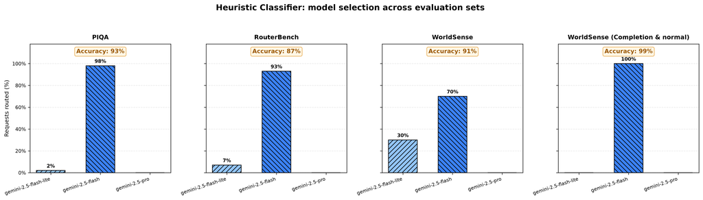
    Model selection by the heuristic classifier across the four evaluation sets, ordered by their assigned reasoning difficulty. Answer accuracy is shown inside each panel. The heuristic predominantly selects gemini-2.5-flash across all four sets and does not select gemini-2.5-pro, resulting in less variation across difficulty levels than the Gemini and Jev classifiers.

    For PIQA, the heuristic routes 2 of the 100 questions to gemini-2.5-flash-lite and 98 to gemini-2.5-flash. The resulting system answers 93 questions correctly. For RouterBench, it routes 7 questions to gemini-2.5-flash-lite and 93 to gemini-2.5-flash. The resulting system answers 87 questions correctly. For WorldSense, the heuristic routes 30 questions to gemini-2.5-flash-lite and 70 to gemini-2.5-flash, producing 91 correct answers. For WorldSense completion and normal, it routes all 100 questions to gemini-2.5-flash, producing 99 correct answers. The heuristic does not select gemini-2.5-pro for any question in the four samples.

    Table 5 reports the complete results. Total evaluation time covers the complete run of 100 questions. All other cost, latency, and token measurements are reported per request.

    Metric
    PIQA
    RouterBench
    WorldSense
    WorldSense, completion and normal
    Accuracy
    93%
    87%
    91%
    99%
    Total evaluation time
    48.7 s
    80.4 s
    56.2 s
    121.0 s
    Model selection [gemini-2.5-flash-lite,
    gemini-2.5-flash,
    gemini-2.5-pro]
    [2%, 98%, 0%]
    [7%, 93%, 0%]
    [30%, 70%, 0%]
    [0%, 100%, 0%]
    Classification cost ($/request)
    0
    0
    0
    0
    Response cost ($/request)
    Mean ± standard deviation
    (range)
    8.60e-04 ± 9.70e-04
    (7.30e-06 to 5.40e-03)
    1.60e-03 ± 1.20e-03
    (1.10e-05 to 6.70e-03)
    1.10e-03 ± 1.30e-03
    (9.10e-06 to 6.80e-03)
    3.00e-03 ± 1.70e-03
    (7.50e-04 to 8.80e-03)
    Response latency (ms)
    Mean ± standard deviation
    (range)
    2,227 ± 2,004
    (629 to 11,413)
    3,787 ± 2,392
    (512 to 14,686)
    2,561 ± 2,321
    (565 to 12,509)
    5,488 ± 2,965
    (1,730 to 14,825)
    Classification latency (ms)
    Mean ± standard deviation
    (range)
    11 ± 8
    (7.8 to 54)
    15 ± 8
    (10 to 49)
    11 ± 7.7
    (6.7 to 44)
    33 ± 99
    (8.4 to 474)
    Output tokens
    Mean ± standard deviation
    (range)
    317 ± 475
    (1 to 3,656)
    636 ± 469
    (1 to 2,644)
    499 ± 596
    (1 to 3,076)
    1,131 ± 692
    (186 to 4,407)

    Table 5. Performance of the heuristic classifier across four evaluation sets, using 100 questions from each set. The heuristic does not invoke a separately billed classification model, so its classification cost is zero. Total evaluation time refers to the complete evaluation run. All other latency, cost, and token measurements are reported per request.

    Classification overhead

    The heuristic has the lowest classification overhead of the three routing strategies. Its mean classification latency ranges from 11 to 33 ms, compared with 235 to 274 ms for Jev and 643 to 720 ms for the Gemini classifier. It also has no separately billed classification cost.

    Low classification overhead does not necessarily produce the lowest response latency or response cost. These measurements also depend on which downstream model the classifier selects. As Figure 3 shows, the heuristic sends most questions in every evaluation set to gemini-2.5-flash.

    Comparison with Jev

    The PIQA results illustrate the distinction between classification overhead and the performance of the complete routed request. The heuristic has a mean classification latency of 11 ms, compared with 235 ms for Jev. However, the heuristic routes 98 questions to gemini-2.5-flash, while Jev routes 93 questions to gemini-2.5-flash-lite.

    In this sample, the heuristic produces 93 correct answers, compared with 89 for Jev. This increase is accompanied by a higher mean response cost and latency. Mean response cost increases from $7.42e-05 with Jev to $8.60e-04 with the heuristic, an increase of more than elevenfold. Mean response latency increases from 1,020 to 2,227 ms.

    On RouterBench, both classifiers produce 87 correct answers. Jev routes 41 questions to gemini-2.5-flash-lite and 59 to gemini-2.5-flash, while the heuristic routes only 7 to gemini-2.5-flash-lite and 93 to gemini-2.5-flash. Jev has a lower mean response cost of $0.0013 per request, compared with $0.0016 for the heuristic. It also has a lower mean response latency of 3,245 ms, compared with 3,787 ms.

    The pattern differs on WorldSense. The heuristic has a lower mean response cost and latency than Jev, but it produces 91 correct answers compared with 97 for Jev. On WorldSense completion and normal, the two classifiers have the same mean response cost. The heuristic produces 99 correct answers, compared with 96 for Jev, and has a slightly lower mean response latency.

    These results do not establish that either classifier is preferable across all evaluation sets. They show that reducing classification overhead alone does not determine the cost, latency, or accuracy of the complete routed request.

    Configuration considerations

    The heuristic provides a low-overhead baseline that is deterministic for a fixed configuration. It also avoids sending a request to a separate classification service. Its results depend on the selected tier boundaries, feature weights, and routing keywords. The default configuration predominantly selects gemini-2.5-flash in these experiments and does not select gemini-2.5-pro. A different configuration could change the model-selection distribution and the resulting accuracy, latency, and cost.

    Unlike Jev, the heuristic does not provide calibrated probabilities or a confidence value that could identify uncertain model selections. Its tier boundaries and scoring rules would therefore need to be evaluated and adjusted using representative application traffic.

    The conclusion compares all three routing strategies across answer accuracy, classification latency, response latency, classification cost, and response cost.

    Conclusions

    Figures 1–3 show that the three classifiers produce substantially different model-selection patterns. The Gemini classifier frequently selects gemini-2.5-pro for the hard WorldSense sets. Jev predominantly selects gemini-2.5-flash for those sets and rarely selects gemini-2.5-pro. The heuristic also favours gemini-2.5-flash, but its model-selection distribution changes less across the four difficulty levels.

    Figure 4 brings the five evaluation metrics together. Each row represents one evaluation set, ordered by its assigned reasoning difficulty. The columns compare answer accuracy, classification latency, response latency, classification cost, and response cost. Each panel contains one bar for the Gemini, Jev, and heuristic classifiers.
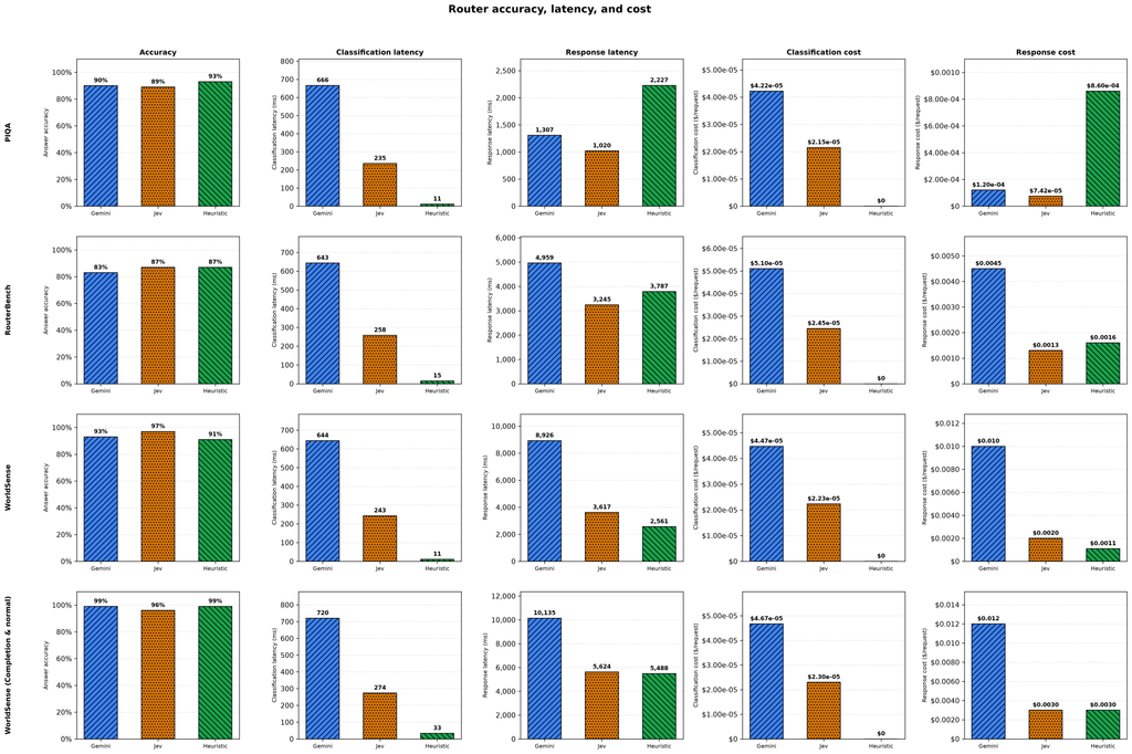
    Answer accuracy, classification latency, response latency, classification cost, and response cost for the Gemini, Jev, and heuristic classifiers across the four evaluation sets. Jev reduces classification latency, response latency, classification cost, and response cost relative to the Gemini classifier on all four sets, while producing higher accuracy on RouterBench and WorldSense and lower accuracy on PIQA and WorldSense completion and normal. The heuristic has the lowest classification overhead, but its response cost, response latency, and accuracy depend on the models selected for each evaluation set.

    Gemini Vs Jev Routing

    Figure 4 shows that Jev has lower classification and response measurements than the Gemini classifier across all four evaluation sets. Mean classification latency with Jev ranges from 235 to 274 ms, compared with 643 to 720 ms for the Gemini classifier. This represents a reduction of approximately 60% to 65%. Jev’s mean classification cost is also approximately half that of the Gemini classifier. The difference continues at the response stage. Compared with the Gemini classifier, Jev reduces mean response cost.

    Jev also reduces mean response latency from 1,307 to 1,020 ms on PIQA, from 4,959 to 3,245 ms on RouterBench, from 8,926 to 3,617 ms on WorldSense, and from 10,135 to 5,624 ms on WorldSense completion and normal.

    These reductions are accompanied by different accuracy results across the evaluation sets. Compared with the Gemini classifier, Jev produces one fewer correct answer on PIQA and three fewer on WorldSense completion and normal. It produces four more correct answers on both RouterBench and WorldSense.

    The Gemini classifier’s higher cost and latency on the WorldSense sets accompany its frequent selection of gemini-2.5-pro. Jev instead routes most questions from these sets to gemini-2.5-flash. The results show that the more frequent use of the reasoning model does not produce higher aggregate accuracy on every evaluation set.

    Jev Vs Heuristic Routing

    The heuristic has the lowest classification latency and no separately billed classification cost. However, Figure 4 shows that reducing classification overhead does not necessarily minimise the cost or latency of the complete routed request. On PIQA, the heuristic produces four more correct answers than Jev, but its mean response cost is more than eleven times higher and its mean response latency is more than twice as high. This difference accompanies the heuristic’s selection of gemini-2.5-flash for 98 questions, while Jev selects gemini-2.5-flash-lite for 93.

    On RouterBench, Jev and the heuristic both produce 87 correct answers. Jev has the lower mean response cost and response latency. It assigns 41 questions to gemini-2.5-flash-lite, compared with 7 under the heuristic. The comparison differs on WorldSense. Jev produces six more correct answers, while the heuristic has lower mean response cost and response latency. On WorldSense completion and normal, the heuristic produces three more correct answers and has slightly lower response latency. Both classifiers have the same mean response cost.

    These results demonstrate that classification overhead is only one component of router performance. The downstream model selected for each request can have a larger effect on response cost and latency than the classification stage itself.

    Conclusion

    Across the five reported metrics, Jev provides best balance across all applicable metrics (accuracy, latency, cost) in our experiments.

    • Jev reduces all four cost and latency measurements relative to the Gemini classifier while maintaining similar aggregate accuracy.
    • Compared with the heuristic, Jev provides lower response cost and latency on PIQA and RouterBench and higher accuracy on WorldSense. The heuristic remains preferable when minimising classification overhead is the primary objective.
    • Jev also provides a confidence value for each classification. This creates the possibility of escalating uncertain requests to a more capable model, but the present experiments do not evaluate such a policy. Confidence thresholds would need to be selected and tested using representative application traffic.

    The experiments also showed distinct differences in the strategy followed by each method:

    • Gemini makes greater use of the more expensive reasoning model, particularly on the two WorldSense sets, resulting in higher response cost and latency.
    • Jev distributes requests mainly between the simple and medium-intelligence models, reducing classification and response overhead while maintaining competitive accuracy.
    • The heuristic eliminates separately billed classification and adds little classification latency, but its strong preference for the medium model can increase response cost on easier questions.

    Limitations

    These findings should be interpreted within the scope of our experiment:

    • Each condition uses 100 sampled questions from each evaluation set.
    • The evaluation uses multiple-choice benchmarks.
    • All downstream models come from one provider (Google) and model family (Gemini).
    • Latency measurements may be affected by external provider load, although we did our best to control for that by timing our experiments.
    • The heuristic uses its default configuration rather than boundaries tuned for our specific experiments.

    Within these limits, the experiments show that request routing can reduce cost and latency without requiring every input to be handled by the most capable model. The central question is not which classifier wins every metric, but which routing strategy provides an acceptable balance of accuracy, latency, and cost for the intended application. In this evaluation, Jev provides the strongest overall balance, while the Gemini and heuristic classifiers remain useful reference points for more conservative and lower-overhead routing strategies, respectively.

    References

    [1] Anastasios Tsourtis. Cost-Aware LLM Request Routing: From Tokenomics to Dynamic Cognitive Allocation. https://research.wpp.com/blog/cost-aware-llm-request-routing-from-tokenomics-to-dynamic-cognitive-allocation

    [2] TypeSafe AI. https://docs.typesafe.ai/

    [3] Daniel Kahneman. Thinking, Fast and Slow. Farrar, Straus and Giroux, 2011.

    [4] LiteLLM https://docs.litellm.ai/docs/proxy/auto_routing#jev-classifier

    [5] PIQA dataset https://inspect.aisi.org.uk/evals/#/eval/piqa

    [6] Worldsense dataset https://inspect.aisi.org.uk/evals/#/eval/worldsense

    [7] Qitian Jason Hu, Jacob Bieker, Xiuyu Li, Nan Jiang, Benjamin Keigwin, Gaurav Ranganath, Kurt Keutzer, and Shriyash Kaustubh Upadhyay. RouterBench: A Benchmark for Multi-LLM Routing System. arXiv:2403.12031, 2024. https://arxiv.org/abs/2403.12031

    [8] Inspect Evals. https://inspect.aisi.org.uk.

  • Cost-Aware LLM Request Routing: From Tokenomics to Dynamic Cognitive Allocation

    Motivation — The Modern Productivity Paradox: LLMflation vs AI bill inflation

    The token, that is the discrete representation of text characters processed by an LLM, is considered as the new economic unit of Artificial Intelligence. Its dual role is unusual: the same object that determines how a model parses and generates information also determines how users are charged and how organizations reason about capacity, utilization and ROI [1].


    Over the past five years, the economics of foundation model inference have followed an aggressive deflationary trajectory of the order of 99.7%, for instance on March 2023 GPT-4: 30$/1M tokens in contrast to 0.1$/1M tokens for frontier open-weight ones by mid-2026. This nominal pricing for LLMs collapsed primarily due to silicon advancements, architectural innovations (Mixture-of-Experts, speculative decoding) and model distillation. This collapse fueled an assumption that machine intelligence was rapidly converging to a zero-marginal-cost commodity. 

    Yet, as enterprises transitioned from isolated proof-of-concept experiments to production deployments, a trend emerged: aggregate AI expenditures surged. Instead of observing deflationary operating bills, enterprises usually face double-digit year-over-year spend increases such as the case of Uber that exhausted the annual budget by April 2026 and Microsoft that cancelled Claude code licences when token bills spiraled out of control ahead of schedule.

    The root cause for this apparent paradox of collapsing pricing and spiking enterprise invoices is not an accounting anomaly. It reflects a shift in how software engineering and deployment consumes machine intelligence. Utilization volume and task complexity surge, shifting consumption from small exploratory queries (such as the static interactive prompts from the early chatGPT days) to continuous background workloads such as  automated reasoning chains (such as the ‘thinking’ part while waiting for a chatbot response) or autonomous pipelines. Consumption exploded precisely because unit prices have fallen (Jevon’s paradox) unmasking an underlying economic reality that enterprises must address to remain profitable and competitive.

    Traditional enterprise software is treated either as: i) capital expenditure or ii) as operational spend: per-seat SaaS subscriptions. In both regimes the cost remains detached from the ‘cognitive throughput it delivers’. In a paper [2] by Microsoft researchers, the authors argue that advanced AI tools cannot be evaluated as passive digital tools as they represent ‘digital labor’ associating autonomous cognitive capabilities that function as independent factors of production alongside human labor. In other words, tokens are not mere bandwidth or storage bytes but a meter of digital labor. Because this metered cognition is embedded across multiple layers of enterprise architecture (from customer-facing applications and internal classification routines to autonomous agentic loops) every single LLM invocation represents an implicit expenditure decision. When enterprises fail to govern this expenditure dynamically, treating every transaction as an unmetered call to the most capable model, the result is runaway operational spend that undermines the very efficiencies generative models promised in the first place.

    The solution: allocating smarter or more economical models based on the background task (or workflow step) complexity, thus optimizing cost instead of always asking for frontier model reasoning at one or two orders of magnitude above what is required.

    Problem Definition — Cost-Aware Request Routing & Agentic Amplification

    To understand why enterprise token consumption defies linear projections, one must examine the architectural evolution of how LLMs are invoked. In traditional human-in-the-loop deployments (e.g., conversational chatbots, inline code completions), token generation is strictly bounded by human pacing. A user submits a query, reviews the output, and formulates a follow-up. In this regime, latency is measured in seconds, sessions terminate when a human pauses, and token consumption scales linearly with user activity. Cost variance is naturally capped by the throughput of the human operator.

    With the introduction of autonomous (multi-step) agentic workflows, inference consumption takes a steep increase. Modern architectures operate largely decoupled from human latency: examples include ReAct, plan-and-solve decompositions and automated reflection loops. A high-level objective such as “reconcile cross-system data discrepancies and generate an audit summary” expands to a recursive loop of many model invocations. In addition, agentic execution introduces context accumulation on every downstream invocation carrying previous responses that grows monotonically. In effect,  what once was a series of discrete/bounded queries is now a compound workload where token volume scales super-linearly across a task. Even worse, multiple tool (code function call) retries, dead-end search paths, chain-of-thought reasoning, memory management (summarization of context before storing to short term memory and transformation of the latter to long term memory [7]) can cause token consumption to surge, requiring the need for budget allocation per business task.

    Simultaneously, the supply side of foundation models has fragmented into specialized capability tiers, ranging from distilled, high-throughput utility ones (often termed -flash or -mini) to massive frontier ones with high test-time reasoning (e.g. Fable 5). Pricing is very differentiated across tiers as well due to performance vs cost trade-off and empirical benchmarks across foundation models demonstrate that it spans from 15x to 100x [6], due to extensive parameter scale, high-memory bandwidth and energy consumption [1]. We suggest that interested reader should consult [1] for a very rigorous analysis on tokenomics, based on model complexity, resource allocation and economic value creation.

    For the scope of this article, we assume that the total inference expenditure into to variables:

    Total cost = Tokens Consumed x price per Token

    (In this case we assume that the input and output token prices are the same, though in general output tokens are more expensive and input token caching is an additional cost). Cost-aware dynamic model routing operates on the unit price multiplier. It would be tempting for developers to route all application traffic to a pinned frontier reasoning model in order to insure against errors or hallucinations. This would lead to burning capital on ‘surplus’ intelligence. On the contrary, naive under-provisioning routing complex tasks involving multi-step reasoning to a budget model induces multi-turn repair cascades due to limited context, hallucinations etc. So the engineering challenge is to decide how to allocate cognition at the request-level and route traffic to the minimum-cost model capable of satisfying the quality constraints. This is the decision layer that evaluates incoming task complexity at real time assisted by tracking telemetry of past decisions (cost, latency, retries).

    Related work on Cost-Aware LLM Routing

    As already described, an LLM router balances performance and cost. Early approaches such as FrugalGPT [6] and AutoMix [8] employ a cascade method which sequentially queries different LLMs until a reliable response is obtained, though this strategy usually needs to query multiple times and leads to high latency. Other cost-aware approaches are: RouteLLM, HybridLLM where queries are directly routed to the most suitable LLM (predictive routing).

    MetaRouter [5] adapts on individual user cost-performance preference feedback by training a policy neural network based on the encoded feedback during an adaptation phase. 

    CoDyn [4] is a code specific LLM router exploring how classifier-based routers specifically evaluate software engineering workloads, proving that a tuned, low-cost router model can match frontier coding capabilities while securing over 43% in code generation savings.

    While tokenomics clarifies why cost-aware allocation is necessary, operationalizing it requires routing algorithms that respect commercial performance commitments. Recent breakthroughs address two core real-world challenges: adapting to sparse feedback and enforcing strict accuracy targets (eg 95% accuracy threshold on critical queries for premium frontier models in contrast to 75% for the corresponding economy tier model). The latter is also referred to as Service Level Agreement (SLA) and it applies on latency besides answer relevance/quality as well.

    PROTEUS [9] is a multi-LLM router that accepts accuracy targets τ as runtime input, in contrast to conventional routers requiring offline hyper-parameter tuning and guessing τ through trial and error, and uses Lagrangian Reinforcement Learning. It employs a learned dual variable λ that tracks constraint violations during training (once) to condition the underlying policy network hence a single trained model can serve the entire accuracy spectrum (τ in [75%, 95%]) dynamically.

    In production systems, where sparse, one-sided feedback is available (meaning that for the training set samples for which a request is dispatched to a given model, the system observes user satisfaction only for that chosen model; counterfactual outcomes for unselected models remain unobserved), SLARouter [3] provides theoretical guarantees for meeting SLA requirements under this relaxed requirement on training data. In addition, SLARouter allows online adaptation as new data arrives so that it can account for distributional drifts, by updating routing boundaries from production data without retraining. Both approaches involve training a small neural network.

    CARROT [11] introduces rate-optimal guarantees but does not adapt online (during inference). Relies on full-feedback datasets and assumes access to data where each query has been evaluated by all available LLMs, that is not always available in real data scenarios.

    Various evaluation benchmarks have been designed to assess the efficiency and accuracy of LLM routers. For instance, RouterBench [10] comprises approximately 405K inference outcomes and includes responses and metrics from 11 distinct LLMs, combining open-source options (like Llama-70B-chat, Mixtral-8x7B-chat, and Mistral-7B) and proprietary systems (like GPT-4 and Claude) as an effort towards a standardized benchmark.

    SPROUT [11] complements RouterBench with 45K queries across 14 models. Together, these benchmarks test complementary aspects: RouterBench provides scale and task diversity (reasoning, factual recall, dialogue, mathematics) with established models, while SPROUT tests generalization to modern model pools with extreme cost variation.

    The progression of request routing reflects a steady shift from rigid developer intuition toward adaptive, SLA-enforceable gateway orchestration. Table 1 summarizes the approaches mentioned so far. This evolutionary trajectory reveals a clear design consensus: high-performance enterprise routing cannot rely solely on static heuristics or opaque third-party black boxes.

    Instead, bridging research and production demands a layered gateway architecture capable of executing sub-millisecond filtering on straightforward traffic while enforcing strict quality and SLA constraints on complex cognitive tasks.

    Routing ParadigmCore Decision MechanismRouting OverheadAdaptivityQuality & SLA Safeguards
    Static / ManualHardcoded model endpoints, prompt prefixes0 msNone (Rigid)Unbounded failure risk on complex queries
    Semantic RoutersVector embedding distance against exemplars50–200 ms(local or hosted encoder, encoder size dependent)Static reference setsHeuristic similarity thresholds without performance bounds
    Cloud Aggregator Routing (e.g., OpenRouter openrouter/auto)Managed proxy heuristics, provider load balancing, and price-tier fallback~25–50 ms (additional proxy latency, Cloudflare edge [12]) + peak hour latency + credit balance checksDynamic provider availability & loadBest-effort provider failover; no formal accuracy floor guarantees
    Predictive Classifiers (e.g., FrugalGPT, RouteLLM)Supervised scoring / fast LLM classification rubric>1000 ms (Encoder size dependent)Offline batch retrainedConfidence scoring; requires per-dataset parameter tuning
    Online SLA Routing (SLARouter)Dual-primal contextual bandit optimizationModernBert Encoder + <1 ms for the MLP classifierOnline (sparse one-sided feedback)Provable probabilistic SLA satisfaction guarantees
    Lagrangian RL Routing (PROTEUS)Policy network conditioned on learned dual variable λ (for online RL training)2.6-8.7ms (based on batching on an A100)Direct runtime input of accuracy target  τStrict floor compliance (Accuracy≥τ) across variable targets
    Hierarchical Hybrid Gateway (LiteLLM Auto Routing)Cascaded Heuristics → Keywords → Fast LLM → Adaptive Pool<1 ms (fast path) to ~50 msThompson Sampling & health metricsMulti-tier failover, fallback chains, and session affinity rails
    Table 1: Model comparison

    LiteLLM – OpenSource, self-hosted, versatile Dynamic Router

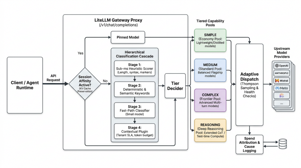
    Having examined the microeconomic foundations of tokenomics and the algorithmic guarantees of SLA-constrained routing, we now outline the architectural blueprint for operationalizing these concepts. Rather than prescribing a fixed code recipe, this section articulates the architectural intent of a dynamic, cost-aware routing layer built upon the open-source LiteLLM Auto Routing framework (Figure 1). LiteLLM is the open source alternative to OpenRouter [12].

    Figure 1: LiteLLM Gateway Proxy Architecture

    The first architectural decision is decoupling application logic from routing intelligence. In standard enterprise codebases, specific models are often hardcoded into agent prompts. This tight coupling complicates failover and prevents cost management. LiteLLM is a central (user managed) AI Gateway providing telemetry and spend attribution to agentic applications by evaluating incoming request complexity and steering execution to the optimal model tier (that is a user-defined pool of comparable models such as ‘cheap’, ‘reasoning’, ‘coding’ etc.).

    The decision (routing) on incoming requests comes with a classification tax: either spending hundreds of milliseconds and tokens on an external LLM to decide or implement a hierarchical classification cascade to resolve requests via low-latency, low-cost mechanisms:

    Stage 1: Heuristic scorer (Fast)
    The gateway inspects structural features of the latest prompt (token length, code syntax tokens, multiple question marks etc) so that zero API calls are made and queries end up immediately to the corresponding model tier in sub-millisecond speed.

    Stage 2: Deterministic & semantic keyword rules (Fast)
    Words in a prompt are matched or approximately matched (fast semantic vector search) to the corresponding tier, for example “hi” → low-cost model, “kubernetes” → reasoning model. In this case the developer can pin a specific model to an agentic tool call.

    Stage 3: (small) LLM classification
    A lightweight, dedicated classifier model such as claude-Haiku or a finetuned and deployed LLM can handle ambiguous requests in order to evaluate their complexity against a structured rubric. Latency can be controlled by a strict timeout so that routing falls under one of the other stages instead.

    Stage 4: Custom classifier plugin

    Custom plugins evaluate organizational metadata such as caller tenant tier (free vs. enterprise SLA), remaining departmental token budgets, or time-of-day cost constraints thus overriding or refining the assigned capability tier before dispatch. This is not about the prompt complexity but rather about a python based instruction allowing more controlled decisions.

    A subtle yet severe failure mode in agentic and multi-turn routing is cache thrashing. Modern model providers offer significant cost discounts (typically 50% to 90%) and latency reductions for input tokens that hit the provider’s Key-Value (KV) prompt cache. If a router evaluates every conversational turn in isolation, Turn 1 might route to Provider A, Turn 2 to Provider B, and Turn 3 back to Provider A. This naive per-turn oscillation invalidates the KV cache on every exchange, forcing full context re-computation, driving up time-to-first-token (TTFT), and inflating aggregate input token costs. LiteLLM incorporates session affinity to track past conversations and pass subsequent turns to the same provider to maximize KV cache hits, when necessary.

    LiteLLM pros:

    • LiteLLM is an opensource (SOC-2 type 2, ISO 27001 certified), proxy server that runs as a container with a db (production features: per key budget limits, cost tracking). Useful for regulated industries in contrast to OpenRouter (3rd party cloud service) where it stores metadata and delegates privacy (training/retention) discretion to the corresponding model provider it internally routes data to. Zero data retention (ZDR) using OpenRouter can be enforced [13] though it might defeat the purpose of (not) choosing a smaller/cheaper model especially considering that this can be achieved with a self-hosted open weight model accessible by LiteLLM.
    • Provides Thompson sampling within models in each tier in order to learn latency distributions between providers and dynamically adapt.
    • Although LiteLLM is another stateful service in the stack in contrast to the fully managed OpenRouter [12] and other variants, we are in control of this important component instead of relying on potential downtimes of a fully managed one. 
    • With respect to latency, LiteLLM adds <1ms (correctly-sized container orchestration, fast caching, logging etc) in contrast to OpenRouter ~25-40ms through its edge network.

    Conclusion & Next Steps — From Pinned Gateways to Dynamic Allocation

    As foundation models evolve from isolated conversational tools into autonomous digital labor, treating machine cognition as an unmetered, monolithic utility is no longer economically sustainable. While macro-level token prices will continue to trend downward, the superlinear token demand driven by multi-step agentic workflows and the growing cost spread between utility and frontier models make dynamic request routing the single most decisive lever for enterprise cost governance.

    The academic literature—from the structural tokenomics of Zhu (2026) to the SLA-constrained algorithms of SLARouter and PROTEUS—proves that intelligent routing can cut inference expenditure by 50% to nearly 90% without compromising task satisfaction. Yet, the ultimate test of these principles lies in their production adoption.

    In our own infrastructure, we have already established the necessary architectural foundation by deploying LiteLLM as a centralized proxy gateway to manage traffic control and cost monitoring across our MultiAgent community [14]. Today, this gateway successfully aggregates credentials, enforces rate limits, and provides unified spend visibility across our active agents. However, our current deployment remains fundamentally predetermined: models are statically pinned to specific agent roles or pipeline tasks. While this ensures predictable execution, it leaves substantial economic efficiency on the table. High-frequency intermediate steps (such as agent handoffs, structured argument extraction, and routine status checks) routinely consume expensive frontier tokens simply because an agent’s assigned model was chosen for its peak cognitive capability rather than its median task requirement.

    Our immediate roadmap focuses on evolving this infrastructure from static model pinning to dynamic, cost-aware cognitive allocation. By transitioning our existing LiteLLM gateway into an active routing intelligence plane, we aim to operationalize the insights of tokenomics research—scaling our multi-agent community with rigorous cost efficiency while preserving frontier reasoning exactly where it matters most.

    Bibliography

    1. [1] Quanyan Zhu (2026). AI Tokenomics: The Economics of Tokens, Computation, and Pricing in Foundation Models. https://arxiv.org/abs/2606.24616
    2. [2] Alex Farach, Alexia Cambon, and Jared Spataro (2025). Evolving the Productivity Equation: Should Digital Labor Be Considered a New Factor of Production? https://arxiv.org/abs/2505.09408
    3. [3] Herbert Woisetschläger, Arastun Mammadli, Ryan Zhang, and Shiqiang Wang (2026). Cost-Optimal LLM Routing with Limited User Feedback under User Satisfaction Guarantees. https://arxiv.org/abs/2606.19376
    4. [4] Mirazul Haque, Petr Babkin, Vali Tawosi, Saba Rahimi, Natraj Raman, Zhiqiang Ma, and Xiaomo Liu (2025). CoDyn: Dynamic LLM Routing for Coding Tasks. NeurIPS 2025 Fourth Workshop on Deep Learning for Code. https://openreview.net/forum?id=0ox03jE6jb
    5. [5] Jiahao Zeng, Ming Tang, and Ningning Ding (2026). Learning to Route LLMs from Implicit Cost-Performance Preferences via Meta-Learning. https://arxiv.org/abs/2606.06178
    6. [6] Lingjiao Chen, Matei Zaharia, and James Zou (2023). FrugalGPT: How to Use Large Language Models While Reducing Cost and Improving Performance. https://arxiv.org/abs/2305.05176
    7. [7] Medium-Tokenomics: FinOps for the Agentic Harness. https://aiadvances.org/tokenomics-for-the-agentic-harness-41dbaa822f7f
    8. [8] Pranjal Aggarwal, Aman Madaan, Ankit Anand, Srividya Pranavi Potharaju, Swaroop Mishra, Pei Zhou, Aditya Gupta, Dheeraj Rajagopal, Karthik Kappaganthu, Yiming Yang, Shyam Upadhyay, Manaal Faruqui, and Mausam (2025). AutoMix: Automatically Mixing Language Models. https://arxiv.org/abs/2310.12963
    9. [9] Amit Singh Bhatti, Vishal Vaddina, and Dagnachew Birru (2026). PROTEUS: SLA-Aware Routing via Lagrangian RL for Multi-LLM Serving Systems. https://arxiv.org/abs/2601.19402
    10. [10] Qitian Jason Hu, Jacob Bieker, Xiuyu Li, Nan Jiang, Benjamin Keigwin, Gaurav Ranganath, Kurt Keutzer, and Shriyash Kaustubh Upadhyay (2024). RouterBench: A Benchmark for Multi-LLM Routing System. https://arxiv.org/abs/2403.12031
    11. [11] Seamus Somerstep, Felipe Maia Polo, Allysson Flavio Melo de Oliveira, Prattyush Mangal, Mírian Silva, Onkar Bhardwaj, Mikhail Yurochkin, and Subha Maity (2025). CARROT: A Cost Aware Rate Optimal Router. https://arxiv.org/abs/2502.03261
    12. [12] OpenRouter (2026). OpenRouter vs LiteLLM: Which LLM Gateway Fits Your Stack? https://openrouter.ai/blog/insights/openrouter-vs-litellm/
    13. [13] OpenRouter (2026). Data Collection. https://openrouter.ai/docs/guides/privacy/data-collection
    14. [14] A research agenda for agent expert communities. https://research.wpp.com/blog/a-research-agenda-for-expert-agent-communities

  • AlphaEvolve Pod: Technical walkthrough

    Marketing teams often struggle to translate past campaign performance data into actionable future decisions. while Neural Network models can help, manual experimentation to improve them is slow, costly, and quickly hits a ceiling. To overcome this, we leveraged AlphaEvolve (AE)—Google DeepMind’s Gemini-powered agentic framework—which autonomously proposes, evaluates, and evolves model architectures in an iterative loop, removing the need for manual trial-and-error. The result: up to 10% improvement in prediction accuracy and up to 7% in recommendation scores over our competitive baselines, achieved in a fraction of the time, and positioning WPP with a first-mover advantage through early access to this technology.

    If you don’t care about the technical details, read our blog post instead.

    Introduction – Scope of this work

    Google AlphaEvolve (AE) [1] is a Gemini-powered agentic framework that reframes model development as an evolutionary search problem. Rather than relying on static optimisation or manual experimentation, AE continuously improves existing algorithms by executing an iterative “generate, test, and refine” loop: at each step, candidate programs are proposed by a large language model, evaluated against a user-defined metric, and fed back into an evolving database of solutions. As a result, the system is capable of autonomously exploring a vast space of model configurations in a semi-supervised manner, without requiring explicit enumeration of all candidate designs.

    The target of this work is to improve two core components of our marketing campaign intelligence pipeline: a prediction model and a recommendation model. Both models had already reached a highly competitive baseline; however, further progress had stalled.

    Despite sustained effort — encompassing bibliographic research, trial-and-error experimentation, and systematic fine-tuning — incremental improvements remained below 1%, and in certain noisy data regimes, accuracy degraded rather than improved. This plateau is particularly consequential in the context of marketing campaign optimisation, where even gains of a few basis points in prediction accuracy can translate into thousands of dollars of savings. Given the scale of the model search space and the cost of manual exploration, AE presents a unique opportunity to dramatically accelerate the discovery of superior model architectures.

    The results of these experiments are compelling. The AE-evolved prediction models achieved an improvement in prediction accuracy of up to 10% over the baseline model. Across both neural and non-neural baselines, as well as fine-tuned Gemma variants, AE-evolved prediction models achieved consistently higher accuracy, validating the hypothesis that evolutionary search can identify architectures that manual experimentation fails to reach in a comparable time frame.

    This report is structured as follows: Section 2 describes how AlphaEvolve works, covering its inputs, inner workings, and output format. Section 3 details the best practices we identified through extensive experimentation. Section 4 describes the base models used as seed programs to be evolved. Section 5 presents and discusses the quantitative results across synthetic and real-world datasets.

    How AE works

    AlphaEvolve is a coding agent that orchestrates a fully autonomous, distributed pipeline of computations — including queries to large language models — to produce algorithms that address a user-specified task. Implemented as an asynchronous pipeline using Python’s asyncio library, the system operates as an evolutionary algorithm: at each iteration, it proposes candidate programs, evaluates them against a target metric, and progressively improves its population of solutions. The result is a search procedure that continuously refines programs toward higher scores without requiring manual intervention between iterations.

    Figure 1 shows the AlphaEvolve pipeline. Note the bidirectional arrow showing that the program database is being used to suggest new programs as well as getting updated with promising solutions through iterations.

    Figure 1 (Image taken from [1]) AlphaEvolve discovery process. The user provides an initial program (with components to evolve marked), evaluation code, and optional configurations. AlphaEvolve then initiates an evolutionary loop. The Prompt sampler uses programs from the Program database to construct rich prompts. Given these prompts, the LLMs generate code modifications (diffs), which are applied to create new programs. These are then scored by Evaluators, and promising solutions are registered back into the Program database, driving the iterative discovery of better and better programs.

    Core pipeline inputs

    Launching an AE experiment requires six key inputs.

    The first is a seed program: an existing, functional codebase with appropriately annotated functions and docstrings, which serves as the starting point for the evolutionary search. AE provides flexibility in its abstraction level, allowing it to tackle problems by either directly evolving the solution itself or by evolving a constructor function that builds the solution (which is often more effective for highly symmetric problems). Users can also provide function templates containing only a detailed docstring and a constant return value, prompting AE to generate the full implementation from scratch.

    The second is a target metric: a scalar value that AE will attempt to maximise iteratively. In our prediction model experiments, we used the macro-average F1-score rather than accuracy, as it proved more effective at steering the search toward better-generalising solutions across imbalanced classes. When multiple metrics are relevant, a weighted linear combination can be used to indirectly optimise them simultaneously.

    The third input is an evaluation function that takes a candidate program and returns the target metric value. Because it is called iteratively to check every new candidate, computational efficiency is critical. In our case, this function fully trains the candidate neural architecture and measures its macro F1-score on a held-out set. The runtime of this function is variable: it depends on the architectural complexity of the candidate (e.g., multi-head attention blocks are slower to compute than linear layers), and because batch size and number of epochs are also subject to evolution, training times can fluctuate significantly across candidates. Early stopping criteria are applied to bound evaluation cost.

    The fourth input is a system prompt that guides the direction of evolution — It provides explicit suggestions on which aspects of the code should be evolved and how, for instance: description of loss functions or search paths to consider. Together with the seed code, the system prompt forms the initial input to the program database sampling process: in effect, it determines both where the search begins and in which direction it is steered.

    The fifth input defines the evolution blocks: contiguous code regions marked with special comments (# EVOLVE-BLOCK-START / # EVOLVE-BLOCK-END) that AE is permitted to modify, while the rest of the codebase remains intact. Carefully scoping these blocks is important — they must be consistent with inter-function dependencies and library imports in the surrounding fixed code. Additional constraints, such as the set of Python libraries available or explicit enumeration of architectural ideas to try, can be incorporated via docstrings or the system prompt.

    The sixth and final input is a stopping criterion — a maximum number of iterations or a target metric threshold — bounds the experiment.

    Inner workings

    At the core of AlphaEvolve is an evolutionary database inspired by the MAP-elites algorithm [2] and island-based population models [3, 4]. Candidate programs and their scores are stored and curated in this database, which is continuously updated as new solutions are evaluated. The database is designed to balance two competing objectives: exploration, by maintaining diversity across the solution space, and exploitation, by prioritising refinement of the highest-scoring programs.

    To generate diverse candidate proposals, AE relies on a mixture of large and small language models — in our experiments, a combination of Gemini 3 Pro and Gemini 3 Flash — which sample from the current program database alongside the seed code and system instructions to produce modified candidate programs. Gemini 3.0 Flash, with its lower latency, enables a higher rate of candidate generation, increasing the volume of ideas explored per unit of time, while Gemini 3.0 Pro provides occasional higher-quality suggestions that can significantly advance the search.

    When an LLM is asked to modify existing code within a larger codebase, it outputs changes as a sequence of SEARCH/REPLACE diff blocks in a structured format — specifying exactly which code segment to replace and with what — allowing for targeted, composable modifications. In cases where the evolved code is very short or a complete rewrite is appropriate, AE can instead instruct the LLM to output the full code block directly.

    Two additional mechanisms further enhance the quality of the search:

    • The first is meta-prompt evolution: AE co-evolves the system prompt itself through a separate LLM step that generates and refines meta-instructions in a dedicated database alongside the candidate programs. This allows the guidance given to the code-generation models to improve over time, potentially surpassing what a human prompter could craft manually — a finding confirmed in ablation experiments reported in the original paper.
    • The second is LLM-generated feedback: beyond the user-provided evaluation function, AE can invoke separate LLM calls to assess qualitative properties of candidate programs that are difficult to measure programmatically, such as code simplicity or readability. These soft scores can steer evolution or filter out undesirable candidates. In our experiments, we observed a beneficial side effect of this mechanism: AE spontaneously added informative comments to complex code segments within evolution blocks that it chose not to modify, improving both readability and the quality of subsequent evolutionary steps.

    Output

    The primary output of an AE experiment is a functional program: a candidate code that achieves the highest target score across all evaluated iterations. Because LLMs occasionally hallucinate, some candidate programs may fail to execute; however, AE handles this gracefully — execution is isolated per candidate, and failed programs are assigned a default score (see next section) while the asynchronous pipeline continues uninterrupted.

    In our experiments, we ran each AE session for up to 1,000 evolutionary iterations, with 4 concurrent candidate evaluations at each step. The final evolved programs, together with all intermediate candidates, can be retrieved post-experiment using their session_id, experiment_id, and program_id identifiers, enabling retrospective inspection of the evolutionary trajectory and diff-level comparison against the seed program.

    Figure 2 Example of an evolution block suggestion. Here AE suggested a parametric non-linear combination of the Cross Entropy loss addressing class imbalance in dataset V17.

    Best practices when using AE

    AlphaEvolve has a shallow entry-point: the user needs only to supply a seed program, an evaluation function, and a maximum number of iterations to launch an experiment. In practice, however, the quality of the outcomes depends strongly on a set of design choices that span prompt engineering, code instrumentation, metric design, and infrastructure planning. Based on our own experiments, we distilled the following guidelines for practitioners.

    1. Invest in the system prompt

    The system prompt is the single most impactful lever available to the user. A prompt that names concrete directions to explore — particular loss families, regularisation strategies, architectural motifs, or hyper-parameter ranges — consistently produces more diverse and higher-scoring candidates than a short, generic instruction. Experimentally, a vague or ambiguous prompt tended to generate overlapping candidate programs with low structural diversity, which hinders the evolutionary search even though AE’s database design is intended to discourage convergence to local minima.

    This observation is corroborated by the paper’s ablation experiments: removing explicit context from the prompt caused a significant drop in discovery performance across both the matrix multiplication and kissing number tasks. Furthermore, AE supports meta-prompt evolution, as we mentioned earlier. In practice, this means the system can progressively improve its own guidance — but this process is seeded by the human-authored prompt, so a strong starting prompt remains essential. Beyond free-text instructions, the prompt can be enriched with explicit context in the form of equations, code snippets, or even PDF attachments of relevant literature.

    2. Place evolution blocks deliberately

    Evolution blocks (delimited by # EVOLVE-BLOCK-START / # EVOLVE-BLOCK-END markers) define the search space (Figure 2). Code outside these markers is treated as a fixed skeleton. Several considerations arise in practice:

    • Scope blocks to the right level of abstraction. AE can evolve a single function, several functions together, or an entire codebase. Broader blocks give AE more latitude but also increase the chance of inconsistencies across function boundaries. Narrower blocks constrain search but keep the skeleton stable.
    • Ensure interface consistency. If the system prompt permits AE to introduce new functions, the evolution block must cover all call sites; otherwise, the fixed code will reference function names that do not exist in the evolved program. This was one of the most common sources of crashing candidates in our experiments.
    • Expose hyper-parameters. Allowing AE to evolve batch size, learning rate, network dimensions, and weight decay treated these as first-class search variables rather than fixed settings. All three of our best-performing variants had hyper-parameters discovered by AE rather than by grid search.
    • Consider the abstraction level carefully. The paper notes that for problems with highly symmetric solutions, evolving a constructor function (which builds the solution from scratch) tends to be more effective than evolving the solution directly. For asymmetric problems — such as our neural architecture — evolving the implementation itself is usually more appropriate, so we opted for that.

    3. Design the evaluation function with care

    The evaluation function is the primary feedback signal for the evolutionary loop. Several properties matter:

    • Speed. Each candidate program must be evaluated before its score can propagate back into the database. Slow evaluations directly limit the number of generations that can be completed within a fixed compute budget. In our case, training a neural network on each candidate introduced variable evaluation times depending on architectural complexity — a cost we accepted in exchange for richer feedback.
    • Default score for failures. If the target metric is non-negative and monotonically increasing, assign a default score of -1 or (-♾️) to candidates that crash or produce invalid output. This prevents degenerate programs from polluting the database with artificially neutral scores.
    • Metric choice. Use a single scalar as the primary optimisation target. For imbalanced classification, we found that positive-class F1-score led to better evolved solutions than accuracy, because it forced AE to address minority-class performance. When multiple qualities matter simultaneously, a weighted linear combination of scalars can be used. Importantly, the paper notes that optimising multiple metrics often improves single-metric results as well: diverse, high-performing programs across different criteria expose the LLMs to a broader solution space, increasing the chance of discovering novel approaches for the target metric.
    • Evaluation cascade. AE supports multi-stage hypothesis testing in which new candidates are first screened on simpler or smaller-scale inputs before being subjected to the full evaluation. This prunes clearly faulty or unpromising programs early and is particularly valuable when full evaluations are expensive. We observed that target scores improved gradually but steadily over hundreds of iterations, with solution complexity increasing as the search matured — a pattern consistent with the cascade’s role in maintaining a healthy exploration–exploitation balance. So run for at least a few hundred iterations. AE’s evolutionary database requires time to accumulate a diverse pool of high-quality programs from which future generations can be sampled.

    4. Manage experiments actively

    • Monitor intermediate candidates. During execution, target scores of successful candidates are visible in real time. Periodically inspecting the diff between the seed program and a high-scoring intermediate candidate — using a tool such as a code editor’s diff view (see Figure 2)— can reveal whether the system prompt is effective, whether evolution blocks are correctly placed, and whether the candidate programs are structurally sound. Early detection of issues saves significant compute.
    • Always verify solutions manually. LLMs can hallucinate plausible-looking but subtly incorrect code. In one of our experiments, a candidate that achieved a high target score did so by inadvertently overfitting: the missing model.eval() / model.train() calls meant that dropout and batch normalisation were applied incorrectly at evaluation time. Human review of the top-performing programs before committing to them is essential.
    • Seed subsequent experiments from the best prior result. Once an experiment concludes, launching a new run seeded with the best-performing program — while retaining the same system prompt — allows AE to continue refining from a strong starting point rather than restarting from the original seed.

    5. Plan infrastructure appropriately

    Choose a Virtual Machine (VM) whose hardware matches the demands of the evaluation function. For neural architecture search, a GPU-accelerated machine substantially reduces per-evaluation training time. More critically, evolved programs can introduce architectural changes — wider layers, additional attention heads, larger batch sizes — that increase memory consumption beyond what the seed program required. Out-of-memory errors during evaluation stall the experiment without providing useful signal. Sizing RAM and VRAM conservatively against the maximum plausible candidate complexity, rather than the seed’s footprint, prevents this failure mode.

    • The user can invoke AE API as another Google Cloud Platform (GCP) service. There is flexibility to call the API (user account with appropriate permissions is set up once) provided that the user is authenticated via gcloud-cli. There are two options to create an experiment: 1) create, start and connect to a virtual machine (VM) on a GCP project, so that cloud resources are utilized (recommended), 2) run locally, using a proprietary machine.

    6. Guard against memory leaks in the fixed code skeleton

    AE executes each candidate program by adding it to an asynchronous queue, where it is run inside the user-provided evaluation function. A key responsibility boundary applies here: AE is only in control of the code inside the evolution blocks. Everything outside — the fixed skeleton, data loading, model initialisation, and the evaluation function itself — is entirely the user’s code and runs as-is for every single candidate evaluation across potentially thousands of iterations.

    This makes memory management in the fixed code important. In our experiments, we encountered a case where a fixed function outside the evolution blocks was not properly releasing memory objects after each evaluation call. Because this code ran once per candidate — and experiments run for hundreds or thousands of iterations — the leak caused memory objects to accumulate steadily, eventually leading to experiment failure.

    To prevent this, we recommend the following hygiene practices for all code outside evolution blocks:

    • Explicitly empty GPU/CPU caches after each evaluation call (e.g. torch.cuda.empty_cache() in PyTorch).
    • Delete intermediate objects that are no longer needed using del, particularly large tensors or model instances created within the evaluation loop.
    • Avoid global variable declarations outside the evaluation function — globals persist across calls and are a common source of unintended object retention.
    • Add explicit garbage collection calls (e.g.import gc; gc.collect()) at the end of the evaluation function, especially when dealing with large objects or when GPU memory is constrained.

    The broader principle is to treat the evaluation function as a self-contained, stateless unit: everything it allocates should be released before it returns.

    7. Choose codebase style

    The codebase can be either self-contained in a Jupyter notebook or in the form a repository-style. In the first case the seed program is provided as a long string whereas in the latter the user indicates the file(s) to be evolved. As mentioned Evolution blocks are indicated by special markers as comments (# EVOLVE-BLOCK-START and # EVOLVE-BLOCK-END). Repository-style codebases are easier to track using version control and by using IDE file diff functionality for the candidate programs.

    Base models

    Prediction model

    The base prediction model is a neural classifier that takes pre-computed feature embeddings as input and assigns each sample to one of three campaign performance classes: positive, average, or negative. Architecturally, it consists of modality-specific encoding layers that project the input embeddings into a lower-dimensional latent space, followed by a fusion layer that combines these projections to produce the final class prediction. Through systematic experimentation across a range of loss functions and their combinations, we identified a weighted mixture of classification and alignment losses as the best-performing training objective. The model is optimised using AdamW (Adam with weight decay) and employs early stopping to prevent overfitting. To rigorously assess the strengths and limitations of each model variant, we constructed a suite of synthetic datasets spanning a range of difficulty levels — varying in complexity, class cardinality, dataset size, and noise level.

    Recommendation model

    The recommendation model is used to ‘fill in the missing puzzle pieces’. A user provides a partial query with missing feature values and the model completes the remaining with appropriate values based on past successful campaign knowledge. The recommendation model relies on the prediction model as an input, where this knowledge is distilled in the model weights. We compile indices for quick look-up and use the top-K recommendations based on approximate K-NN search in the projection latent space. A design decision was to run separate, independent optimisation experiments for each model rather than a joint optimisation, making sequential rather than simultaneous optimisation the natural approach. For the synthetic datasets where the ground truth known and represented as a graph, we devised a metric to score the success of good candidates. This metric considers empty recommendations and at the same time penalizes for low-performing ones. We refer to the normalized value of this metric as avg norm score (Table 3).

    Results

    Inspecting the top performing prediction programs

    We present the main points for the three top performing AE programs of multiple experiments for the prediction model. Table 1 summarizes the differences with the base program (seed).

    • Upon launching a plethora of AE experiments using different input datasets and refining the system prompt accordingly, we chose three best performing variants and use the naming convention Centroid_Loss, Cross_Modal_Attn and Focal_Loss henceforth (Table 1).
    • All three AE-discovered variants abandoned the base model’s shared encoder design, opting instead for separate, identical encoders for each input modality — suggesting the evolutionary search consistently converged on specialised, non-shared representations that were initially used to balance network capacity with data size.
    • Each variant introduced a distinct custom loss function replacing the base contrastive loss: Centroid_Loss uses Centroid Loss, Cross_Modal_Attn uses a Hyper-spherical centroid loss (used for inter-sample and intra-sample alignment), and Focal_Loss a Cosine Centroid Attraction loss (on the positive class) — indicating that loss function innovation was the primary lever AE exploited to improve performance.
    • Cross_Modal_Attn introduced the most complex architectural changes: Beyond the loss, Cross_Modal_Attn added a gating layer on the encoder, label smoothing, and an entanglement-based classifier with cross-modal attention — making it the most structurally different from the base model among the three. On the contrary,Centroid_Loss focused on regularisation and normalisation refinements: Its changes (layer norms and different activation functions) are relatively conservative compared to Cross_Modal_Attn/Focal_Loss, suggesting that even lightweight, targeted modifications discovered by AE can yield meaningful gains.
    • Cross_Modal_Attn and Focal_Loss also introduced architectural innovations beyond the loss, with Cross_Modal_Attn adding a gating layer on the encoder and an entanglement-based classifier with modal attention, and Focal_Loss incorporating Focal loss (targeting class imbalance) and batch normalisation in the classifier — showing AE’s ability to co-evolve both loss and architecture simultaneously.
    • Hyper-parameter tuning was itself part of the evolved solution: all three variants had learning rate and network dimensions evolved by AE, while Centroid_Loss and Focal_Loss additionally evolved weight decay (optimizer) — demonstrating that AE treated hyper-parameters as first-class search variables, not just fixed settings. We should note here that hyper-parameter tuning on our base model was done using grid search.
    • The three variants were evolved on different target datasets (Centroid_Loss & Cross_Modal_Attn on V16, Focal_Loss on V17), reflecting a deliberate strategy of running separate AE experiments tailored to datasets of varying difficulty, rather than a single universal optimisation. Nevertheless Centroid_Loss and Cross_Modal_Attn performance is similar accross datasets (Table 2) indicating robustness.
    base modelCentroid_LossCross_Modal_AttnFocal_Loss
    encoder layershared + dedicated for GEOseparate identical encodersseparate identical encodersseparate identical encoders
    extra Losscontrastive with marginCentroid LossHyper-spherical centroid lossCosine Centroid Attraction loss
    changes–layernorm’sgating layer on encoder, label smoothing in LossFocal loss (for class imbalance)
    ClassifierMLPdifferent activation functionsLR, network dimsadded batch normalization
    Hyper-param tuninggrid searchLR, network dims, weight decayentanglement-based with cross-modal AttentionLR, network dims, weight decay
    Target dataset–V16V16V17
    Table 1 Prediction model best performing variants discovered using AlphaEvolve. Base model: our own proprietary model serving as seed model. Centroid_Loss, Cross_Modal_Attn, Focal_Loss belong to separate AE experiments where they reached the highest target score after hundreds of iterations.

    Results on Prediction

    datasetmetricbase modelCentroid_LossCross_Modal_AttnFocal_Loss
    V15avg F1-score90.22%92.65%93.09%89.60%
    easy, imbalancedNEG F1-score90.45%92.20%92.12%90.70%
    AVE F1-score97.50%98.02%98.16%96.85%
    POS F1-score82.89%87.74%88.99%81.25%
    extra V16avg F1-score78.40%85.92%85.72%71.22%
    med, imbalancedNEG F1-score71.57%81.30%80.54%59.91%
    AVE F1-score95.00%96.53%96.41%88.79%
    POS F1-score68.61%79.92%80.20%64.96%
    V17avg F1-score30.32%30.34%33.33%34.91%
    hard, imbalancedNEG F1-score0%0%0.26%15.83%
    AVE F1-score90.98%90.97%90.04%63.50%
    POS F1-score0%0.06%9.70%25.39%
    V25avg F1-score86.48%89.75%89.48%81.65%
    balancedNEG F1-score89.37%91.30%91.30%87.42%
    AVE F1-score82.78%86.66%86.16%71.79%
    POS F1-score87.30%91.28%90.98%85.73%
    V26avg F1-score85.28%89.11%87.68%79.30%
    balancedNEG F1-score89.75%91.11%88.88%83.49%
    AVE F1-score80.90%86.02%84.43%67.46%
    POS F1-score85.18%90.22%89.71%86.95%
    Realavg F1-score63.00%71.00%71.12%57.44%
    imbalancedNEG F1-score52.00%63.74%62.78%56.53%
    AVE F1-score82.00%85.21%85.37%59.70%
    POS F1-score56.00%64.33%65.20%56.10%
    Accuracy72.00%77.11%77.37%57.75%
    Table 2 Prediction model score comparison across dataset and model variants. Base model: seed model, var. Results are reported as: macro-average f1 (avg f1-score) and per-class f1-score (NEG, POS, AVE). Centroid_Loss and Cross_Modal_Attn are consistently well performing across datasets and all variants outperform the base model. The standard deviation of reported means is ± 0.005%.

    Key Findings

    • AE-evolved variants consistently outperform the already well-performing base model across almost all datasets and metrics: Centroid_Loss and Cross_Modal_Attn show gains on V15, V16, V25, and V26, confirming that AE’s evolutionary search reliably identifies architectures superior to our baseline.
    • Cross_Modal_Attn is the best performer on easy/medium synthetic data (V15, V16): It leads on avg F1 for V15 (93.09% vs. base 90.22%) and ties Centroid_Loss on V16 (85.72% vs. 85.92%), while also achieving the highest POS F1 on V16 (80.20% vs. base 68.61%) — a striking +11.6pp improvement on the hardest-to-classify minority class.
    • Focal_Loss is uniquely effective on the hardest dataset (V17): While the base model and Centroid_Loss score 0% on both NEG and POS F1 (essentially collapsing to a degenerate classifier), Focal_Loss achieves 15.83% NEG and 25.39% POS F1 — breaking through a performance floor that the other variants could not overcome.
    • The minority class (NEG/POS) gains are consistently larger than the average class (AVE) gains: For example on V16, the base AVE F1 is already 95.00% and Centroid_Loss only improves it to 96.53%, whereas POS F1 jumps from 68.61% to 80.20%. This pattern repeats across datasets, indicating AE’s variants are particularly effective at addressing class imbalance. This is particularly important as correct identification of the positive class (well performing campaigns) is critical for the recommendation model.
    • Centroid_Loss and Cross_Modal_Attn show similar and robust performance across datasets: Despite being evolved independently on V16, both variants score comparably on V15, V16, V25, and V26, suggesting AE converged on a similarly generalizable solution space from different starting conditions — evidence of stability in the evolutionary search.
    • Centroid_Loss is the strongest all-round performer on balanced/moderate synthetic data (V25, V26): It leads avg F1 on both V25 (89.75% vs. base 86.48%) and V26 (89.11% vs. base 85.28%), consistently outperforming Cross_Modal_Attn and Focal_Loss on these datasets. On the contrary Focal_Loss underperforms on all datasets except V17, suggesting it was over-specialised for the hard imbalanced regime and does not generalise well to easier distributions.
    • Gains on real data are the most practically significant: On the real-world imbalanced dataset, Centroid_Loss achieves a +8pp avg F1 (71% vs. 63%), +11.74pp NEG F1 (63.74% vs. 52%), +8.33pp POS F1 (64.33% vs. 56%), and +5.11pp accuracy (77.11% vs. 72%) — the largest absolute improvements across all tested datasets, validating that AE’s gains hold on actual production data. Cross_Modal_Attn attains a comparable improvement as well.

    Results on Recommendation

    datasetmetricbase Predictor/ base RecommenderAE Predictor/ base RecommenderAE Predictor/ AE Recommender

    V15
    easy, imbalanced
    avg normalized score0.43580.46410.5019

    V16
    med, imbalanced
    avg normalized score0.30940.33970.3973
    V17 hard, imbalancedavg normalized score0.00.29150.3615
    V25 balancedavg normalized score0.51010.57930.6055
    V26 balancedavg normalized score0.51690.55350.5857
    Table 3 | Recommendation model score comparison across dataset and model variants. The average normalized score is based on the ground truth graph and penalizes for negative/empty recommendations (higher is better). Base Predictor is the base model from Table 1. AE Predictor is the best AE model, for each dataset (Table 2). AE Recommender is the best AE-evolved candidate based on our Recommendation model. There is incremental improvement by combining the AE candidate Prediction and Recommendation models.

    Key Findings

    • Combining AE-evolved components at both stages yields the strongest results across all datasets: The fully AE pipeline (AE Predictor / AE Recommender) consistently achieves the highest average normalised score on every tested dataset — 0.5019 on V15, 0.3973 on V16, and 0.3615 on V17 — confirming that gains from prediction and recommendation evolution are additive.
    • The AE Predictor alone delivers meaningful gains over the baseline pipeline: Even when paired with the base Recommender, replacing the base Predictor with its AE-evolved counterpart improves the normalised score by +6.5% on V15 (0.4358 → 0.4641), +9.8% on V16 (0.3094 → 0.3397), and lifts V17 from a score of 0.0 to 0.2915 — demonstrating that prediction quality is a critical upstream bottleneck for recommendation performance.
    • The hardest dataset (V17) shows the most dramatic absolute improvement: The base pipeline scores 0.0 on V17, meaning it produces no valid recommendations under the most challenging data regime. The AE Predictor alone breaks this failure floor (0.2915), and the fully AE pipeline extends it further to 0.3615.
    • The recommendation model benefits from AE evolution beyond what better predictions alone provide: On all three datasets, the jump from (AE Predictor / base Recommender) to (AE Predictor / AE Recommender) is consistent and substantial — +0.0378 on V15, +0.0576 on V16, +0.0700 on V17 — indicating that the recommendation model itself harbours independent optimisation headroom that AE successfully exploits.
    • Gains scale with dataset difficulty: The absolute improvement of the fully AE pipeline over the all-base baseline increases as difficulty grows — +0.0661 on V15, +0.0879 on V16, and +0.3615 on V17 (from zero). This suggests AE’s evolutionary search is particularly valuable in challenging, noisy data regimes where conventional optimisation approaches stall.

    Conclusion

    • The results are compelling: the evolved models achieved an improvement in prediction accuracy of up to 10% over the baseline model.
    • Prediction: No single variant dominates across all datasets: Cross_Modal_Attn leads on V15, Centroid_Loss leads on V25/V26/Real, and Focal_Loss is indispensable for V17 — implying that for a production deployment spanning diverse data regimes, an ensemble or dataset-aware model selection strategy would be optimal.
    • Recommendation: The evolved prediction model alone delivers meaningful gains over the base Recommendation. Combining the best prediction and Recommendation models improves recommendation scores even further.

    This project was a collaboration between the WPP Research team including: Anastasios Tsourtis and Theodoros Lappas and the AI for Science team at Google Cloud including (but not limited to): Kartik Sanu, Laurynas Tamulevičius, Nicolas Stroppa, Chris Page, Gary Ng, John Semerdjian, Skandar Hannachi, Vishal Agarwal, and Anant Nawalgaria, Gabriela Hernandez Larios and partners at Google DeepMind

    References

    1. Novikov, A., Vũ, N., Eisenberger, M., Dupont, E., Huang, P.-S., Wagner, A. Z., Shirobokov, S., Kozlovskii, B., Ruiz, F. J. R., Mehrabian, A., Kumar, M. P., See, A., Chaudhuri, S., Holland, G., Davies, A., Nowozin, S., Kohli, P., & Balog, M. (2025). AlphaEvolve: A coding agent for scientific and algorithmic discovery. arXiv:2506.13131 [cs.AI]. https://arxiv.org/abs/2506.13131
    2. Mouret, J.-B., & Clune, J. (2015). Illuminating search spaces by mapping elites. arXiv:1504.04909 [cs.AI]. https://arxiv.org/abs/1504.04909
    3. Romera-Paredes, B., Barekatain, M., Novikov, A., Balog, M., Kumar, M. P., Dupont, E., Ruiz, F. J. R., Ellenberg, J. S., Wang, P., Fawzi, O., Kohli, P., & Fawzi, A. (2024). Mathematical discoveries from program search with large language models. Nature, 625(7995), 468–475. https://doi.org/10.1038/s41586-023-06924-6
    4. Tanese, R. (1989). Distributed genetic algorithms for function optimization. University of Michigan.
  • Cracking the Code of Campaign Success with Google’s AlphaEvolve Agent

    In the fast-paced world of digital marketing, one deceptively simple question keeps resurfacing: “What knowledge can we extract from successful past campaigns to make better future marketing decisions?”

    Every brand sits on a goldmine of historical campaign data: thousands of images, videos, and overall campaign configurations that either soared or sank. The challenge isn’t a lack of information; it’s injecting that knowledge at the precise moment the next decision is being made. How do we operationalise lessons learned to answer questions like:

    • Prediction
      “Given Brand A, the target region of São Paulo, a set of creatives featuring outdoor sports imagery, and audience group of millennials aged 25–34, how well is the campaign expected to perform? “
    • Recommendation
      “Given Brand B and a target region of Milan, what should the creatives (videos/images) look like to maximise engagement among environmentally conscious consumers aged 15–18?”

    A common suggestion is to simply “ask an AI.” While modern Large Language Models (LLMs) are remarkably capable and encode broad real-world knowledge, they lack the tribal knowledge embedded in your proprietary data. They don’t know your specific brand voice, your audience’s unique quirks, or the subtle patterns behind your past failures. To truly win, you need a system that learns from your history—the hits, the misses, and everything in between.

    To address this, the WPP Research invests significant effort in developing prediction and recommendation models trained on large and diverse volumes of historical campaign data. These models are highly competitive and continuously improving. However, at some point during development, progress inevitably hits a plateau: even incremental gains—rarely exceeding 1%—demand extensive bibliographic research, days or even weeks of trial-and-error experimentation, and painstaking fine-tuning.

    With time at a premium, a vast space of possible improvements to explore (architectural changes, hyperparameter tuning), and experiments that are inherently slow to run, we turned to Google’s AlphaEvolve (AE) [1]: a Gemini-powered agentic framework that reframes model development as an evolutionary search problem. Rather than relying on manual experimentation, AlphaEvolve autonomously proposes, evaluates, and refines candidate model architectures in an iterative loop, guided by the expertise of our Data Science team and grounded in objective performance metrics.

    The results are striking: what weeks of manual experimentation struggled to improve by a single percentage point, AlphaEvolve achieved in a fraction of the time, delivering prediction accuracy gains of up to 10% on both synthetic and real datasets, while simultaneously lifting downstream recommendation scores up to 7%.

    Our access to AlphaEvolve came through Google’s Early Access Program (EAP), within the context of the ongoing partnership between Google and the WPP Research. Throughout our adventures with AlphaEvolve, we have been collaborating closely with the Google Research team, providing and receiving feedback. This collaboration has been invaluable to the project’s success.

    The AlphaEvolve Advantage

    Building a good AI model is painfully slow. A team of experts reads through mountains of research papers, rewrites code by hand, and runs experiments that can take days, only to find the improvement is tiny, or worse, a dead end. This research → code → test → repeat cycle creates a huge gap between having data and actually getting value from it.

    And even after you pick a model architecture, you still have to tune it. Think of it like adjusting the equalizer on a stereo: dozens of sliders, each affecting the sound, and you’re trying to find the perfect combination by ear. Techniques like grid search and Bayesian optimization help, but they’re still limited by what the human designer guesses might work. Not what the data actually needs. Trying every possible combination? Far too expensive and slow.

    The honest truth is that the search space is simply too vast for human intuition and trial-and-error to navigate. This is exactly where AlphaEvolve (AE) changes the game.

    Instead of a person manually tweaking one model at a time, AE treats the entire development process as an evolutionary search. Much like natural selection, but for code. It generates candidate models as functional programs, runs them, and scores each one against a target metric. It doesn’t just tune models. It designs them from scratch.

    Under the hood, AE is powered by Google’s state-of-the-art Gemini model, working hand-in-hand with a curated program database from Google DeepMind. Together, they explore millions of possible code configurations, zeroing in on the most accurate solution that meets our constraints. A search of this breadth would take a human team months. AlphaEvolve does it in a fraction of the time.

    By shifting from manual experimentation to this autonomous framework, we don’t just speed things up. We uncover strategies and architectures that human intuition alone would never find. Figure 3 illustrates this iterative loop in action.

    Figure 3 AlphaEvolve is a Gemini-powered coding agent from Google that automatically improves algorithms through a “generate, test, and refine” loop. The user provides three inputs: a description of the problem, a way to score candidate solutions, and a starting program to build from. AlphaEvolve then proposes many code variations using Gemini, scores each one automatically, and keeps the best-performing ideas—recombining and evolving them over multiple rounds, much like natural selection. With each cycle, the solutions get sharper, often surpassing what the original starting point could achieve.

    Guided Evolution: The Human in the Loop

    AlphaEvolve is autonomous, but it is not unsupervised. Think of it as digital evolution: the AI proposes ideas and keeps only the winners to build upon in the next generation. This process still requires careful navigation by our Data Scientists, who provide clear system instructions and constraints to guide the search through an infinite landscape of potential improvements, while inspecting for deviations introduced by the stochastic nature of LLMs. The result is a search that stays focused on logical, high-quality architectures and respects the real-world boundaries of the problem we are addressing.

    In the example below, we illustrate the inputs that AE expects from the human in the loop, as well as the output that it produces.

    Input 1: A System prompt describing the problem and steer evolution towards search directions.

    An example system prompt is: “Evolve a training model for a neural network 3-class classifier that achieves high accuracy on a provided dataset. The model must consist of a loss function that… . Focus on the multi-objective optimization of the following scores… Consider changing the model architecture to include…”

    Think of the System Prompt as the instruction manual you hand to AlphaEvolve before it starts work. Imagine hiring a highly skilled but very literal engineer. They’re brilliant, but they need a clear, written brief to work from — they won’t assume anything. The System Prompt is that brief. It channels AlphaEvolve’s enormous computational power toward the right problem, in the right direction. It covers:

    • What the job is — e.g., “Build a model that can classify campaign outcomes into three categories.”
    • What the rules are — constraints it must respect, such as how the input data is structured or what the model architecture must look like.
    • Where to focus — specific areas to explore and improve, for example: “Try changing the loss function”.
    • What success looks like — the specific performance goals it should be optimising for (e.g., accuracy scores). This is also why the human expertise of the Data Science team remains critical.

    Input 2: A Seed Program with an initial solution that you hand to AlphaEvolve to improve.

    Rather than asking AlphaEvolve to build something from scratch, you give it a model that already works — and ask it to make it better. The team deliberately marks which parts AlphaEvolve is permitted to experiment with (using special labels in the code), and which parts must remain untouched. The Seed Program represents the accumulated expertise and investment already put into your AI models. AlphaEvolve doesn’t throw that away — it builds on top of it. It’s the difference between renovating a solid building versus demolishing it and starting over.

    Input 3: The Target metric that AE will attempt to maximise in order to achieve our objective.

    The Target Metric is essentially how the business defines “better.” This is a critical decision made by the Data Science team — not the AI. If the metric is well-chosen, AlphaEvolve will find solutions that genuinely deliver business value. If it’s poorly defined, the AI could optimize for the wrong thing entirely. Imagine you’re running a sales team and you’ve set a clear goal: maximise the conversion rate. Every change your team tries — new pitch, new pricing, new outreach method — gets evaluated against that one number. If a change improves the conversion rate, you keep it. The Target Metric works exactly the same way for AlphaEvolve. It might be something like “predict campaign performance as accurately as possible” — expressed as a single numerical score. AlphaEvolve runs each candidate model, checks the score, and keeps only the ones that do better. So the Target Metric is the objective, measurable definition of what winning looks like.

    Input 4: The Stopping criteria.

    The Stopping Criteria is simply the pre-agreed rule for when to call it done. Since AlphaEvolve could theoretically keep running and experimenting forever, the team sets clear boundaries upfront for when the experiment should end. A maximum number of rounds — e.g., “Run up to 500 iterations, then stop.” A performance threshold — e.g., “Stop as soon as the model reaches 90% accuracy.” This is like saying: “Once we’ve hit our goal, there’s no need to keep going.”

    Output: a ranked list of improved AI models.

    Figure 4 shows a ‘before’ (left) and ‘after’ (right) comparison of a section of a seed program that AlphaEvolve was asked to improve. Changes are highlighted in green. We observe several changes:

    • Training parameters were upgraded. For example, the number of training cycles (EPOCHS) was increased, the model’s internal size (PROJ_DIM) grew and a regularisation setting (WEIGHT_DECAY) was adjusted. These are the kind of fine-tuning decisions that would normally take a data scientist considerable time and experimentation to arrive at.
    • The model’s internal logic was redesigned. The component responsible for processing data (the “encoder”) was restructured and even renamed to better reflect its purpose. AlphaEvolve didn’t just tweak numbers. It proposed a more sophisticated architecture. New techniques were introduced.
    Figure 4 Example of an evolved block of code where AE is permitted to modify the contents of this segment. The function contents are modified and changes in names are reflected in other code blocks appropriately. Note that training parameter values are suggested as well indicating compatible architectural changes with hyperparameter tuning.

    Results: does it actually work?

    AlphaEvolve was applied to two core problems:

    • Performance Prediction, which estimates a campaign’s performance based on its configuration.
    • Performance-aware recommendation, which suggests the optimal way to complete/update a campaign’s configuration, in order to maximise its performance.

    Both models had already reached a highly competitive baseline with further manual improvements stalling below 1%.

    Datasets

    We evaluated all models on a suite of six datasets: five synthetic (details using an internally developed pipeline can be found here) and one real-world. This yielded datasets spanning a range of regimes: easy/medium/hard, depending on the noise profile and class balance – classes with a fewer samples are characterized as minority. Easy and imbalanced (V15), medium and imbalanced (V16), hard and imbalanced (V17), medium and balanced (V25, V26). The real-world dataset consists of actual historical campaign records and serves as the ultimate validation of whether gains observed on synthetic data transfer to production conditions.

    Prediction

    Three top-performing AE-evolved variants (Centroid_Loss, Cross_Modal_Attn, Focal_Loss) were identified across multiple experiments. All three consistently outperformed the base model across synthetic and real-world datasets.

    In order to asses the model performance we use the industry standard F1 score that is a way of measuring how good a model is at classification (class ‘POS’ is high-performing, class ‘NEG’ is low-performing, class ‘AVG’ average-performing) , balancing two things: Precision — “When the model says something is positive, how often is it right?” Recall — “Out of all the actual positives, how many did the model catch?” If the model is good at one but terrible at the other, the F1 score will be low. We calculate the F1 score separately for each class (NEG, AVE, POS), then take the plain average avg F1-score.

    • On easy/medium synthetic data (V15, V16): Cross_Modal_Attn achieved the strongest overall performance, reaching 93.09% avg F1-score on V15 (vs. 90.22% baseline) and a striking +11.6 percentage point improvement on the hardest-to-classify minority class POS on V16 (POS F1: 80.20% vs. 68.61%).
    • On the hardest synthetic dataset (V17): Focal_Loss broke through a performance floor that other variants could not — the base model scored 0% on both minority classes (NEG and POS), while Focal_Loss achieved 15.83% and 25.39% respectively.
    • On real-world data: Centroid_Loss delivered the most practically significant gains — +8pp avg F1 (71% vs. 63%), +11.74pp NEG F1, +8.33pp POS F1, and +5.11pp accuracy — validating that AE’s improvements hold on actual production data.

    Across all datasets and variants, gains on minority classes (correctly identifying hig-performing and low-performing campaigns) were consistently larger than gains on the majority class — a particularly valuable outcome given that minority-class accuracy is the critical input for the recommendation model.

    Recommendation

    The recommendation model, which relies on the prediction model’s outputs, was evaluated both in isolation and in a fully evolved end-to-end pipeline. The recommendation score (higher is better) is a metric that measures how good the recommendations are by comparing them against a known “ground truth” (applicable to synthetic datasets). It rewards recommendations that correctly identify high-performing campaign configurations, whereas it penalizes two kinds of failures: i) empty (the model couldn’t suggest anything) ii) of low-quality (the model suggested something, but it performs poorly).

    • Swapping in the AE-evolved predictor alone improved recommendation scores meaningfully: +6.5% on easy data (V15), +9.8% on medium data (V16), and lifted the hard dataset (V17) from a score of 0.0 (which essentially means that all recommendations were wrong) to 0.29.
    • Combining the AE-evolved predictor with an AE-evolved recommender produced the strongest results across all datasets, with the fully evolved pipeline achieving scores of 0.5 (V15), 0.4 (V16), and 0.36 (V17) — confirming that the gains from prediction and recommendation evolution are additive.
    • Recommendation improvements of up to 7% were observed when both components were evolved together.

    Conclusion

    AlphaEvolve works — and it works exceptionally well. It represents a meaningful and measurable step forward in model development. Applied to WPP AI Lab’s campaign prediction and recommendation models, which had already reached a performance plateau through conventional means, AlphaEvolve delivered prediction accuracy gains of up to 10% on both synthetic and real datasets, while simultaneously lifting downstream recommendation scores by up to 7%. It surfaces architectural strategies and configurations that lie beyond the reach of human intuition alone, not by replacing the expertise of our Data Science team, but by amplifying it. The human-in-the-loop dynamic remains essential: our scientists shape the search space, define meaningful constraints, and validate the outputs.

    AlphaEvolve does the heavy lifting of exploration. As prediction and recommendation models continue to grow in complexity, AlphaEvolve offers a glimpse of a future where the gap between data collection and model improvement is measured in hours rather than weeks, and where the best-performing systems are not just built by experts, but co-designed with AI.

    This project was a collaboration between the WPP Research team including: Anastasios Tsourtis and Theodoros Lappas and the AI for Science team at Google Cloud including (but not limited to): Kartik Sanu, Laurynas Tamulevičius, Nicolas Stroppa, Chris Page, Gary Ng, John Semerdjian, Skandar Hannachi, Vishal Agarwal, and Anant Nawalgaria, Gabriela Hernandez Larios and partners at Google DeepMind

    References

    1. Novikov, A., Vũ, N., Eisenberger, M., Dupont, E., Huang, P.-S., Wagner, A. Z., Shirobokov, S., Kozlovskii, B., Ruiz, F. J. R., Mehrabian, A., Kumar, M. P., See, A., Chaudhuri, S., Holland, G., Davies, A., Nowozin, S., Kohli, P., & Balog, M. (2025). AlphaEvolve: A coding agent for scientific and algorithmic discovery. arXiv:2506.13131 [cs.AI]. https://arxiv.org/abs/2506.13131

    Ready to explore the specifics? Read our full technical deep dive into the technical report for a closer look at our methodology.

    Disclaimer: This content was created with AI assistance. All research and conclusions are the work of the WPP Research team.